Fit SOPDT with Regression
 |  |  |  |
|---|
A second-order linear system with time delay is an empirical description of potentially oscillating dynamic processes. These systems are common in chemical processes, mechanical systems, and other applications where the output response can exhibit overshoot and oscillations before reaching a steady state.
The general form of the SOPDT model is given by:
$$\tau_s^2 \frac{d^2y}{dt^2} + 2 \zeta \tau_s \frac{dy}{dt} + y = K_p \, u\left(t-\theta_p \right)$$
where:
- `y(t)` is the output variable (e.g., temperature, concentration, position).
- `u(t)` is the input variable (e.g., heater power, feed rate, force).
- `K_p` is the process gain, representing the steady-state change in output per unit change in input.
- `\tau_s` is the second-order time constant, representing the speed of response.
- `\zeta` is the damping factor, determining the degree of oscillation in the response.
- `\theta_p` is the time delay (dead time), representing a delay between the input change and the output response.
Understanding SOPDT Parameters
Each parameter in the SOPDT model significantly influences the system's dynamic behavior:
- Process Gain (`K_p`): Indicates how much the output will eventually change for a unit change in input. A higher gain results in a larger steady-state output.
- Second-Order Time Constant (`\tau_s`): Determines the speed of the system's response. A smaller time constant means a faster response to input changes.
- Damping Factor (`\zeta`):
- Overdamped (`\zeta > 1`): The system returns to steady state without oscillations but slower.
- Critically Damped (`\zeta = 1`): Fastest return to steady state without oscillations.
- Underdamped (`0 < \zeta < 1`): The system oscillates before settling at the steady state.
- Time Delay (`\theta_p`): Represents the delay between an input change and the system's initial response. Common in processes with transport or communication delays.
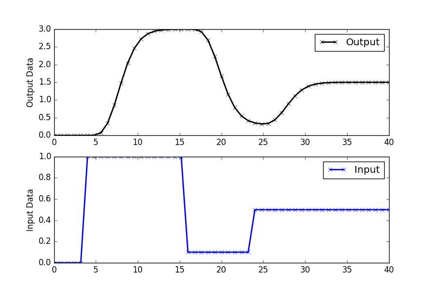
Simulated Data from the SOPDT Model
To demonstrate how to fit an SOPDT model to data, generate simulated data using a higher-order process model. The simulated data mimics real process behavior, including the dynamic response to changes in the input variable.

import numpy as np
import matplotlib.pyplot as plt
from scipy.integrate import odeint
# Define a higher-order process model to generate data
def process(y, t, n, u, Kp, taup):
"""
Higher-order process model (nth-order system)
"""
dydt = np.zeros(n)
# First derivative
dydt[0] = (-y[0] + Kp * u) / (taup / n)
# Higher-order derivatives
for i in range(1, n):
dydt[i] = (-y[i] + y[i - 1]) / (taup / n)
return dydt
# Time points
ns = 100 # Number of time steps
t = np.linspace(0, 40, ns)
delta_t = t[1] - t[0]
# Input vector (piecewise constant input)
u = np.zeros(ns)
u[5:20] = 1.0
u[20:30] = 0.1
u[30:] = 0.5
def sim_process_data():
"""
Simulate the process data using the higher-order process model.
"""
n = 10 # Order of the system
Kp = 2.5 # Process gain
taup = 5.0 # Process time constant
yp = np.zeros(ns) # Initialize output array
y0 = np.zeros(n) # Initial conditions
for i in range(ns - 1):
ts = [t[i], t[i + 1]]
args = (n, u[i], Kp, taup)
y = odeint(process, y0, ts, args=args)
y0 = y[-1]
yp[i + 1] = y[-1][n - 1]
return yp
yp = sim_process_data()
# Save data to a file
data = np.vstack((t, u, yp)).T
np.savetxt('data_sopdt.txt', data, delimiter=',', comments='', header='time,u,y')
# Plot the simulated data
plt.figure(figsize=(10, 6))
plt.subplot(2, 1, 1)
plt.plot(t, yp, 'k-', linewidth=2, label='Output y(t)')
plt.ylabel('Output')
plt.legend(loc='best')
plt.subplot(2, 1, 2)
plt.plot(t, u, 'b-', linewidth=2, label='Input u(t)')
plt.ylabel('Input')
plt.xlabel('Time')
plt.legend(loc='best')
plt.tight_layout()
plt.show()
SOPDT Fit to Data
Estimate the SOPDT model parameters (`K_p`, `\tau_s`, `\zeta`, `\theta_p`) that best fit the process data. We use optimization techniques to minimize the sum of squared errors (SSE) between the model predictions and the observed data.
Below are two methods to perform the parameter estimation:
- Scipy Optimization Tools
- GEKKO Optimization Suite
Method 1: SOPDT Fit Using Scipy
import pandas as pd
import matplotlib.pyplot as plt
from scipy.integrate import odeint
from scipy.optimize import minimize
from scipy.interpolate import interp1d
import warnings
# Import CSV data file
# Column 1 = time (t)
# Column 2 = input (u)
# Column 3 = output (yp)
url = 'http://apmonitor.com/pdc/uploads/Main/data_fopdt.txt'
data = pd.read_csv(url)
t = data['time'].values - data['time'].values[0]
u = data['u'].values
yp = data['y'].values
u0 = u[0]
y0 = yp[0]
xp0 = yp[0]
# specify number of steps
ns = len(t)
delta_t = t[1]-t[0]
# create linear interpolation of the u data versus time
uf = interp1d(t,u)
def sopdt(x,t,uf,Kp,taus,zeta,thetap):
# Kp = process gain
# taus = second order time constant
# zeta = damping factor
# thetap = model time delay
# ts^2 dy2/dt2 + 2 zeta taus dydt + y = Kp u(t-thetap)
# time-shift u
try:
if (t-thetap) <= 0:
um = uf(0.0)
else:
um = uf(t-thetap)
except:
# catch any error
um = u0
# two states (y and y')
y = x[0] - y0
dydt = x[1]
dy2dt2 = (-2.0*zeta*taus*dydt - y + Kp*(um-u0))/taus**2
return [dydt,dy2dt2]
# simulate model with x=[Km,taum,thetam]
def sim_model(x):
# input arguments
Kp = x[0]
taus = x[1]
zeta = x[2]
thetap = x[3]
# storage for model values
xm = np.zeros((ns,2)) # model
# initial condition
xm[0] = xp0
# loop through time steps
for i in range(0,ns-1):
ts = [t[i],t[i+1]]
inputs = (uf,Kp,taus,zeta,thetap)
# turn off warnings
with warnings.catch_warnings():
warnings.simplefilter("ignore")
# integrate SOPDT model
x = odeint(sopdt,xm[i],ts,args=inputs)
xm[i+1] = x[-1]
y = xm[:,0]
return y
# define objective
def objective(x):
# simulate model
ym = sim_model(x)
# calculate objective
obj = 0.0
for i in range(len(ym)):
obj = obj + (ym[i]-yp[i])**2
# return result
return obj
# initial guesses
p0 = np.zeros(4)
p0[0] = 3 # Kp
p0[1] = 5.0 # taup
p0[2] = 1.0 # zeta
p0[3] = 2.0 # thetap
# show initial objective
print('Initial SSE Objective: ' + str(objective(p0)))
# optimize Kp, taus, zeta, thetap
solution = minimize(objective,p0)
# with bounds on variables
#no_bnd = (-1.0e10, 1.0e10)
#low_bnd = (0.01, 1.0e10)
#bnds = (no_bnd, low_bnd, low_bnd, low_bnd)
#solution = minimize(objective,p0,method='SLSQP',bounds=bnds)
p = solution.x
# show final objective
print('Final SSE Objective: ' + str(objective(p)))
print('Kp: ' + str(p[0]))
print('taup: ' + str(p[1]))
print('zeta: ' + str(p[2]))
print('thetap: ' + str(p[3]))
# calculate model with updated parameters
ym1 = sim_model(p0)
ym2 = sim_model(p)
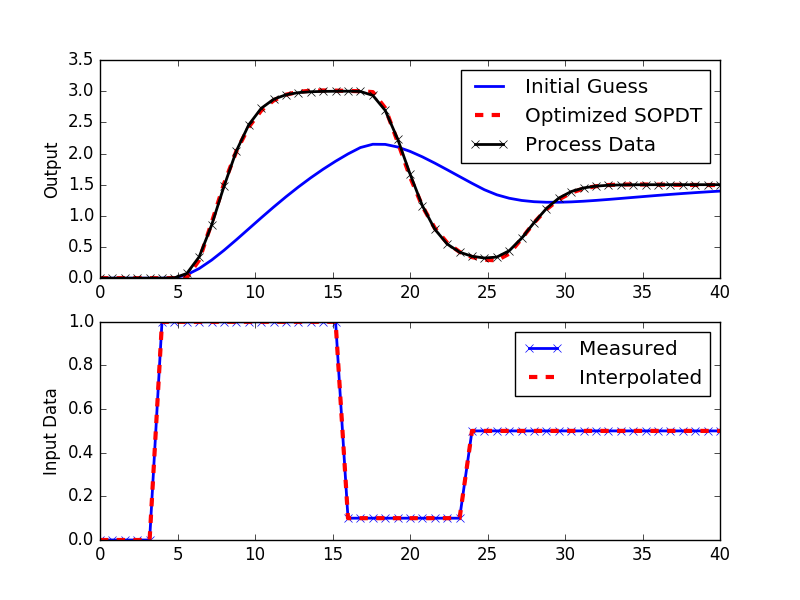
# plot results
plt.figure()
plt.subplot(2,1,1)
plt.plot(t,ym1,'b-',linewidth=2,label='Initial Guess')
plt.plot(t,ym2,'r--',linewidth=3,label='Optimized SOPDT')
plt.plot(t,yp,'k--',linewidth=2,label='Process Data')
plt.ylabel('Output')
plt.legend(loc='best')
plt.subplot(2,1,2)
plt.plot(t,u,'bx-',linewidth=2)
plt.plot(t,uf(t),'r--',linewidth=3)
plt.legend(['Measured','Interpolated'],loc='best')
plt.ylabel('Input Data')
plt.savefig('results.png')
plt.show()
Method 2: SOPDT Fit Using GEKKO
GEKKO is an optimization suite that facilitates model building and solving differential equations.
import pandas as pd
from gekko import GEKKO
import matplotlib.pyplot as plt
# Import CSV data file
# Column 1 = time (t)
# Column 2 = input (u)
# Column 3 = output (y)
url = 'http://apmonitor.com/pdc/uploads/Main/data_sopdt.txt'
data = pd.read_csv(url)
t = data['time'].values - data['time'].values[0]
u = data['u'].values
y = data['y'].values
m = GEKKO(remote=False)
m.time = t; time = m.Var(0); m.Equation(time.dt()==1)
K = m.FV(2,lb=0,ub=10); K.STATUS=1
tau = m.FV(3,lb=1,ub=200); tau.STATUS=1
theta_ub = 30 # upper bound to dead-time
theta = m.FV(0,lb=0,ub=theta_ub); theta.STATUS=1
zeta = m.FV(1,lb=0.1,ub=3); zeta.STATUS=1
# add extrapolation points
td = np.concatenate((np.linspace(-theta_ub,min(t)-1e-5,5),t))
ud = np.concatenate((u[0]*np.ones(5),u))
# create cubic spline with t versus u
uc = m.Var(u); tc = m.Var(t); m.Equation(tc==time-theta)
m.cspline(tc,uc,td,ud,bound_x=False)
ym = m.Param(y); yp = m.Var(y); xp = m.Var(y)
m.Equation(xp==yp.dt())
m.Equation((tau**2)*xp.dt()+2*zeta*tau*yp.dt()+yp==K*(uc-u[0]))
m.Minimize((yp-ym)**2)
m.options.IMODE=5
m.solve(disp=False)
print('Kp: ', K.value[0])
print('taup: ', tau.value[0])
print('thetap: ', theta.value[0])
print('zetap: ', zeta.value[0])
# plot results
plt.figure()
plt.subplot(2,1,1)
plt.plot(t,y,'k.-',lw=2,label='Process Data')
plt.plot(t,yp.value,'r--',lw=2,label='Optimized SOPDT')
plt.ylabel('Output')
plt.legend()
plt.subplot(2,1,2)
plt.plot(t,u,'b.-',lw=2,label='u')
plt.legend()
plt.ylabel('Input')
plt.show()
Fit SOPDT Model to Experimental Data
In this example, we fit an SOPDT model to real experimental data from a temperature control lab (TCLab). The TCLab is a device with a heater and a temperature sensor, exhibiting second-order dynamics due to thermal mass and heat transfer effects.
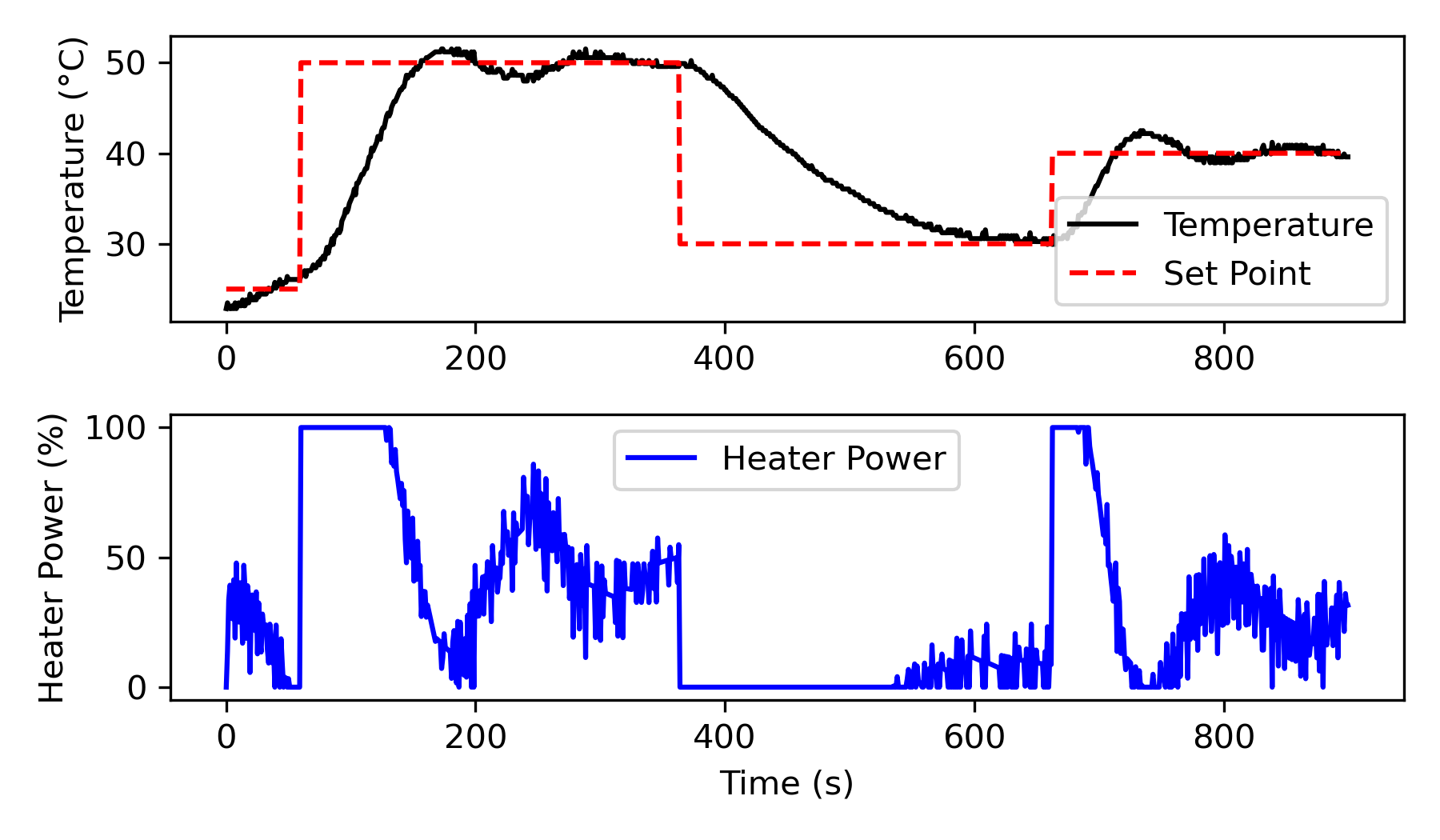
Generating Experimental Data
Run the TCLab by applying step changes in the temperature set point and record the heater, temperature, and set point over time.
import numpy as np
import time
import matplotlib.pyplot as plt
from scipy.integrate import odeint
######################################################
# Use this script for evaluating model predictions #
# and PID controller performance for the TCLab #
# Adjust only PID and model sections #
######################################################
######################################################
# PID Controller #
######################################################
# inputs -----------------------------------
# sp = setpoint
# pv = current temperature
# pv_last = prior temperature
# ierr = integral error
# dt = time increment between measurements
# outputs ----------------------------------
# op = output of the PID controller
# P = proportional contribution
# I = integral contribution
# D = derivative contribution
def pid(sp,pv,pv_last,ierr,dt):
Kc = 15.0 # K/%Heater
tauI = 40.0 # sec
tauD = 1.0 # sec
# Parameters in terms of PID coefficients
KP = Kc
KI = Kc/tauI
KD = Kc*tauD
# ubias for controller (initial heater)
op0 = 0
# upper and lower bounds on heater level
ophi = 100
oplo = 0
# calculate the error
error = sp-pv
# calculate the integral error
ierr = ierr + KI * error * dt
# calculate the measurement derivative
dpv = (pv - pv_last) / dt
# calculate the PID output
P = KP * error
I = ierr
D = -KD * dpv
op = op0 + P + I + D
# implement anti-reset windup
if op < oplo or op > ophi:
I = I - KI * error * dt
# clip output
op = max(oplo,min(ophi,op))
# return the controller output and PID terms
return [op,P,I,D]
# save txt file with data and set point
# t = time
# u1,u2 = heaters
# y1,y2 = tempeatures
# sp1,sp2 = setpoints
def save_txt(t, u1, u2, y1, y2, sp1, sp2):
data = np.vstack((t, u1, u2, y1, y2, sp1, sp2)) # vertical stack
data = data.T # transpose data
top = ('Time,Q1,Q2,T1,T2,SP1,SP2')
np.savetxt('data.txt', data, delimiter=',', header=top, comments='')
######################################################
# FOPDT model #
######################################################
Kp = 0.5 # degC/%
tauP = 120.0 # seconds
thetaP = 10 # seconds (integer)
Tss = 23 # degC (ambient temperature)
Qss = 0 # % heater
######################################################
# Energy balance model #
######################################################
def heat(x,t,Q):
# Parameters
Ta = 23 + 273.15 # K
U = 10.0 # W/m^2-K
m = 4.0/1000.0 # kg
Cp = 0.5 * 1000.0 # J/kg-K
A = 12.0 / 100.0**2 # Area in m^2
alpha = 0.01 # W / % heater
eps = 0.9 # Emissivity
sigma = 5.67e-8 # Stefan-Boltzman
# Temperature State
T = x[0]
# Nonlinear Energy Balance
dTdt = (1.0/(m*Cp))*(U*A*(Ta-T) \
+ eps * sigma * A * (Ta**4 - T**4) \
+ alpha*Q)
return dTdt
######################################################
# Do not adjust anything below this point #
######################################################
# Connect to Arduino
a = tclab.TCLab()
# Turn LED on
print('LED On')
a.LED(100)
# Run time in minutes
run_time = 15.0
# Number of cycles
loops = int(60.0*run_time)
tm = np.zeros(loops)
# Temperature
# set point (degC)
Tsp1 = np.ones(loops) * 25.0
Tsp1[60:] = 50.0
Tsp1[360:] = 30.0
Tsp1[660:] = 40.0
T1 = np.ones(loops) * a.T1 # measured T (degC)
error_sp = np.zeros(loops)
Tsp2 = np.ones(loops) * 23.0 # set point (degC)
T2 = np.ones(loops) * a.T2 # measured T (degC)
# Predictions
Tp = np.ones(loops) * a.T1
error_eb = np.zeros(loops)
Tpl = np.ones(loops) * a.T1
error_fopdt = np.zeros(loops)
# impulse tests (0 - 100%)
Q1 = np.ones(loops) * 0.0
Q2 = np.ones(loops) * 0.0
print('Running Main Loop. Ctrl-C to end.')
print(' Time SP PV Q1 = P + I + D')
print(('{:6.1f} {:6.2f} {:6.2f} ' + \
'{:6.2f} {:6.2f} {:6.2f} {:6.2f}').format( \
tm[0],Tsp1[0],T1[0], \
Q1[0],0.0,0.0,0.0))
# Create plot
plt.figure() #figsize=(10,7)
plt.ion()
plt.show()
# Main Loop
start_time = time.time()
prev_time = start_time
dt_error = 0.0
# Integral error
ierr = 0.0
try:
for i in range(1,loops):
# Sleep time
sleep_max = 1.0
sleep = sleep_max - (time.time() - prev_time) - dt_error
if sleep>=1e-4:
time.sleep(sleep-1e-4)
else:
print('exceeded max cycle time by ' + str(abs(sleep)) + ' sec')
time.sleep(1e-4)
# Record time and change in time
t = time.time()
dt = t - prev_time
if (sleep>=1e-4):
dt_error = dt-1.0+0.009
else:
dt_error = 0.0
prev_time = t
tm[i] = t - start_time
# Read temperatures in Kelvin
T1[i] = a.T1
T2[i] = a.T2
# Simulate one time step with Energy Balance
Tnext = odeint(heat,Tp[i-1]+273.15,[0,dt],args=(Q1[i-1],))
Tp[i] = Tnext[1]-273.15
# Simulate one time step with linear FOPDT model
z = np.exp(-dt/tauP)
Tpl[i] = (Tpl[i-1]-Tss) * z \
+ (Q1[max(0,i-int(thetaP)-1)]-Qss)*(1-z)*Kp \
+ Tss
# Calculate PID output
[Q1[i],P,ierr,D] = pid(Tsp1[i],T1[i],T1[i-1],ierr,dt)
# Start setpoint error accumulation after 1 minute (60 seconds)
if i>=60:
error_eb[i] = error_eb[i-1] + abs(Tp[i]-T1[i])
error_fopdt[i] = error_fopdt[i-1] + abs(Tpl[i]-T1[i])
error_sp[i] = error_sp[i-1] + abs(Tsp1[i]-T1[i])
# Write output (0-100)
a.Q1(Q1[i])
a.Q2(0.0)
# Print line of data
print(('{:6.1f} {:6.2f} {:6.2f} ' + \
'{:6.2f} {:6.2f} {:6.2f} {:6.2f}').format( \
tm[i],Tsp1[i],T1[i], \
Q1[i],P,ierr,D))
# Plot
plt.clf()
ax=plt.subplot(4,1,1)
ax.grid()
plt.plot(tm[0:i],T1[0:i],'r.',label=r'$T_1$ measured')
plt.plot(tm[0:i],Tsp1[0:i],'k--',label=r'$T_1$ set point')
plt.ylabel('Temperature (degC)')
plt.legend(loc=2)
ax=plt.subplot(4,1,2)
ax.grid()
plt.plot(tm[0:i],Q1[0:i],'b-',label=r'$Q_1$')
plt.ylabel('Heater')
plt.legend(loc='best')
ax=plt.subplot(4,1,3)
ax.grid()
plt.plot(tm[0:i],T1[0:i],'r.',label=r'$T_1$ measured')
plt.plot(tm[0:i],Tp[0:i],'k-',label=r'$T_1$ energy balance')
plt.plot(tm[0:i],Tpl[0:i],'g-',label=r'$T_1$ linear model')
plt.ylabel('Temperature (degC)')
plt.legend(loc=2)
ax=plt.subplot(4,1,4)
ax.grid()
plt.plot(tm[0:i],error_sp[0:i],'r-',label='Set Point Error')
plt.plot(tm[0:i],error_eb[0:i],'k-',label='Energy Balance Error')
plt.plot(tm[0:i],error_fopdt[0:i],'g-',label='Linear Model Error')
plt.ylabel('Cumulative Error')
plt.legend(loc='best')
plt.xlabel('Time (sec)')
plt.draw()
plt.pause(0.05)
# Turn off heaters
a.Q1(0)
a.Q2(0)
# Save text file
save_txt(tm[0:i],Q1[0:i],Q2[0:i],T1[0:i],T2[0:i],Tsp1[0:i],Tsp2[0:i])
# Save figure
plt.savefig('test_PID.png')
# Allow user to end loop with Ctrl-C
except KeyboardInterrupt:
# Disconnect from Arduino
a.Q1(0)
a.Q2(0)
print('Shutting down')
a.close()
save_txt(tm[0:i],Q1[0:i],Q2[0:i],T1[0:i],T2[0:i],Tsp1[0:i],Tsp2[0:i])
plt.savefig('test_PID.png')
# Make sure serial connection still closes when there's an error
except:
# Disconnect from Arduino
a.Q1(0)
a.Q2(0)
print('Error: Shutting down')
a.close()
save_txt(tm[0:i],Q1[0:i],Q2[0:i],T1[0:i],T2[0:i],Tsp1[0:i],Tsp2[0:i])
plt.savefig('test_PID.png')
raise
Note: Optionally replace 'tclab_pid.csv' URL with your experimental data file generate from the script above.
import matplotlib.pyplot as plt
# Load experimental data
#file = 'tclab_pid.csv'
file = 'http://apmonitor.com/pdc/uploads/Main/tclab_pid.csv'
data = pd.read_csv(file)
t_exp = data['Time'].values
u_exp = data['Q1'].values
y_exp = data['T1'].values
sp = data['SP1'].values
# Plot the experimental data
plt.figure(figsize=(6, 3.5))
plt.subplot(2, 1, 1)
plt.plot(t_exp, y_exp, 'k-', label='Temperature')
plt.plot(t_exp, sp, 'r--', label='Set Point')
plt.ylabel('Temperature (°C)')
plt.legend()
plt.subplot(2, 1, 2)
plt.plot(t_exp, u_exp, 'b-', label='Heater Power')
plt.ylabel('Heater Power (%)')
plt.xlabel('Time (s)')
plt.legend()
plt.tight_layout()
plt.savefig('tclab_pid.png',dpi=300)
plt.show()
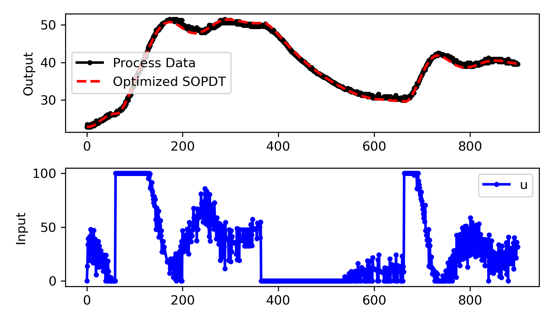
Fit the SOPDT Model to Experimental Data
We use the same fitting approach as before but apply it to the experimental data.
import pandas as pd
from gekko import GEKKO
import matplotlib.pyplot as plt
# Load experimental data
#file = 'tclab_pid.csv'
file = 'http://apmonitor.com/pdc/uploads/Main/tclab_pid.csv'
data = pd.read_csv(file)
t = data['Time'].values - data['Time'].values[0]
u0 = data['Q1'].values[0]
y0 = data['T1'].values[0]
u = data['Q1'].values - u0
y = data['T1'].values - y0
m = GEKKO(remote=False)
m.time = t; time = m.Var(0); m.Equation(time.dt()==1)
K = m.FV(2,lb=0,ub=1); K.STATUS=1
tau = m.FV(3,lb=1,ub=200); tau.STATUS=1
theta_ub = 30 # upper bound to dead-time
theta = m.FV(0,lb=0,ub=theta_ub); theta.STATUS=1
zeta = m.FV(1,lb=0.5,ub=3); zeta.STATUS=1
# add extrapolation points
td = np.concatenate((np.linspace(-theta_ub,min(t)-1e-5,5),t))
ud = np.concatenate((u[0]*np.ones(5),u))
# create cubic spline with t versus u
uc = m.Var(u); tc = m.Var(t); m.Equation(tc==time-theta)
m.cspline(tc,uc,td,ud,bound_x=False)
ym = m.Param(y); yp = m.Var(y); xp = m.Var(y)
m.Equation(xp==yp.dt())
m.Equation((tau**2)*xp.dt()+2*zeta*tau*yp.dt()+yp==K*(uc-u[0]))
m.Minimize((yp-ym)**2)
m.options.IMODE=5
m.solve(disp=False)
print('Kp: ', K.value[0])
print('taup: ', tau.value[0])
print('thetap: ', theta.value[0])
print('zetap: ', zeta.value[0])
# plot results
plt.figure(figsize=(6,3.5))
plt.subplot(2,1,1)
plt.plot(t,y+y0,'k.-',lw=2,label='Process Data')
plt.plot(t,yp.value+y0,'r--',lw=2,label='Optimized SOPDT')
plt.ylabel('Output')
plt.legend()
plt.subplot(2,1,2)
plt.plot(t,u+u0,'b.-',lw=2,label='u')
plt.legend()
plt.ylabel('Input')
plt.tight_layout()
plt.savefig('pid_data_SOPDT.png',dpi=300)
plt.show()
Discussion of Results
The SOPDT model parameters provide insights into the system dynamics.
- Process Gain (`K_p`=0.64): Indicates how much the temperature changes per unit change in heater power.
- Time Constant (`\tau_s`=45.7 sec): Reflects the speed of the temperature response.
- Damping Factor (`\zeta`=1.83): Determines whether the temperature overshoots the setpoint.
- Time Delay (`\theta_p`=4.5 sec): Accounts for the delay between heater activation and temperature change.
Is the damping factor for the heater / temperature response overdamped, critically damped, or underdamped?
- Overdamped `(\zeta>1)`
- Critically damped `(\zeta=1)`
- Underdamped `(0 \le \zeta < 1)`
Comparing the model output with the experimental data helps validate the model accuracy and identify any discrepancies.
Conclusion
Fitting an SOPDT model to process data captures the essential dynamics of a system with potential oscillatory behavior and time delays. The estimated model can be used for controller design, simulation studies, and understanding system behavior.