Quiz: Transient Balance Equations
 |  |  |  |
|---|
1. You precisely measure the beginning and end weight of an unknown reaction in a sealed container. The results indicate a net loss of mass. Which of the following are possibilities? Select all that are correct.
- Correct. Incorrect weight measurements can be a possible source of error.
- Correct. Measurement noise is a possible source of random variation in the results. The noise can be caused by electromagnetic interference, precision limits on the analog to digital converter, or power supply voltage fluctuations. One way to characterize measurement noise and precision is to take repeated measurements and report the average and distribution.
- Correct. A small amount of mass is converted into energy with nuclear fission or fusion. Chemical reactions are not nuclear reactions because changes in chemical compounds and bonds do not influence the nucleus of an atom.
- Incorrect. Even though the reaction may have released heat or increased the pressure, the mass inside the container is still constant. Mass is conserved so an increase in species or kinetic energy does not influence the weight.
- Incorrect. The gravitational constant decreases with increased elevation. The mass is the same but the weight may be less if the measurement is taken at a higher elevation relative to the starting measurement.
2. What is the correct mass balance with variable volume and liquid density?
$$\frac{dm}{dt} = \frac{d(\rho\,V)}{dt} = \sum \dot m_{i} - \sum \dot m_{o}$$
- Incorrect. The density changes. It is not a constant to bring out of the derivative term.
- Incorrect. The volume changes. It is not a constant to bring out of the derivative term.
- Correct. This is the correct form because `\rho` and `V` are both variable. The chain rule is used to divide combined terms `\frac{d(\rho V)}{dt}`.
- Incorrect. You cannot split `\frac{d(\rho V)}{dt}` this way. Use the chain rule instead.
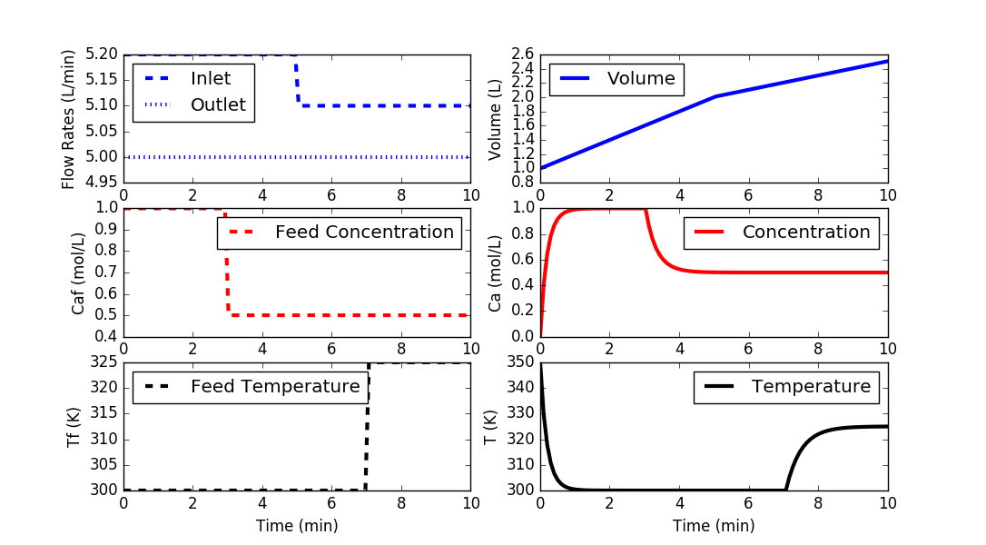
3. The source code for a blending simulation is given in the following code.

import matplotlib.pyplot as plt
from scipy.integrate import odeint
# define mixing model
def vessel(x,t,q,qf,Caf,Tf):
# Inputs (4):
# qf = Inlet Volumetric Flowrate (L/min)
# q = Outlet Volumetric Flowrate (L/min)
# Caf = Feed Concentration (mol/L)
# Tf = Feed Temperature (K)
# States (3):
# Volume (L)
V = x[0]
# Concentration of A (mol/L)
Ca = x[1]
# Temperature (K)
T = x[2]
# Parameters:
# Reaction
rA = 0.0
# Mass balance: volume derivative
dVdt = qf - q
# Species balance: concentration derivative
# Chain rule: d(V*Ca)/dt = Ca * dV/dt + V * dCa/dt
dCadt = (qf*Caf - q*Ca)/V - rA - (Ca*dVdt/V)
# Energy balance: temperature derivative
# Chain rule: d(V*T)/dt = T * dV/dt + V * dT/dt
dTdt = (qf*Tf - q*T)/V - (T*dVdt/V)
# Return derivatives
return [dVdt,dCadt,dTdt]
# Initial Conditions for the States
V0 = 1.0
Ca0 = 0.0
T0 = 350.0
y0 = [V0,Ca0,T0]
# Time Interval (min)
t = np.linspace(0,10,100)
# Inlet Volumetric Flowrate (L/min)
qf = np.ones(len(t))* 5.2
qf[50:] = 5.1
# Outlet Volumetric Flowrate (L/min)
q = np.ones(len(t))*5.0
# Feed Concentration (mol/L)
Caf = np.ones(len(t))*1.0
Caf[30:] = 0.5
# Feed Temperature (K)
Tf = np.ones(len(t))*300.0
Tf[70:] = 325.0
# Storage for results
V = np.ones(len(t))*V0
Ca = np.ones(len(t))*Ca0
T = np.ones(len(t))*T0
# Loop through each time step
for i in range(len(t)-1):
# Simulate
inputs = (q[i],qf[i],Caf[i],Tf[i])
ts = [t[i],t[i+1]]
y = odeint(vessel,y0,ts,args=inputs)
# Store results
V[i+1] = y[-1][0]
Ca[i+1] = y[-1][1]
T[i+1] = y[-1][2]
# Adjust initial condition for next loop
y0 = y[-1]
# Construct results and save data file
data = np.vstack((t,qf,q,Tf,Caf,V,Ca,T)) # vertical stack
data = data.T # transpose data
np.savetxt('data.txt',data,delimiter=',')
# Plot the inputs and results
plt.figure()
plt.subplot(3,2,1)
plt.plot(t,qf,'b--',linewidth=3)
plt.plot(t,q,'b:',linewidth=3)
plt.ylabel('Flow Rates (L/min)')
plt.legend(['Inlet','Outlet'],loc='best')
plt.subplot(3,2,3)
plt.plot(t,Caf,'r--',linewidth=3)
plt.ylabel('Caf (mol/L)')
plt.legend(['Feed Concentration'],loc='best')
plt.subplot(3,2,5)
plt.plot(t,Tf,'k--',linewidth=3)
plt.ylabel('Tf (K)')
plt.legend(['Feed Temperature'],loc='best')
plt.xlabel('Time (min)')
plt.subplot(3,2,2)
plt.plot(t,V,'b-',linewidth=3)
plt.ylabel('Volume (L)')
plt.legend(['Volume'],loc='best')
plt.subplot(3,2,4)
plt.plot(t,Ca,'r-',linewidth=3)
plt.ylabel('Ca (mol/L)')
plt.legend(['Concentration'],loc='best')
plt.subplot(3,2,6)
plt.plot(t,T,'k-',linewidth=3)
plt.ylabel('T (K)')
plt.legend(['Temperature'],loc='best')
plt.xlabel('Time (min)')
plt.show()
Adjust the simulation to have step changes Inlet flow = 5.5 L/min and Feed Temperature = 315 K. Start the changes at 3 minutes of simulation time. With these changes, what is the concentration at 4 minutes?
- Correct. You modified the simulation correctly.
- Incorrect. This is the concentration at 0.4 min.
- Incorrect. This is the result if you don't include the step changes.
- Incorrect. Print Ca[40] for the exact value.
