Solve Differential Equations in Python
Differential equations can be solved with different methods in Python. Below are examples that show how to solve differential equations with (1) GEKKO Python, (2) Euler's method, (3) the ODEINT function from Scipy.Integrate. Additional information is provided on using APM Python for parameter estimation with dynamic models and scale-up to large-scale problems.
1. GEKKO Python
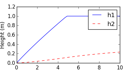
See Introduction to GEKKO for more information on solving differential equations in Python. GEKKO Python solves the differential equations with tank overflow conditions. When the first tank overflows, the liquid is lost and does not enter tank 2. The model is composed of variables and equations. The differential variables (h1 and h2) are solved with a mass balance on both tanks.
import matplotlib.pyplot as plt
from gekko import GEKKO
m = GEKKO()
# integration time points
m.time = np.linspace(0,10)
# constants
c1 = 0.13
c2 = 0.20
Ac = 2 # m^2
# inflow
qin1 = 0.5 # m^3/hr
# variables
h1 = m.Var(value=0,lb=0,ub=1)
h2 = m.Var(value=0,lb=0,ub=1)
overflow1 = m.Var(value=0,lb=0)
overflow2 = m.Var(value=0,lb=0)
# outflow equations
qin2 = m.Intermediate(c1 * h1**0.5)
qout1 = m.Intermediate(qin2 + overflow1)
qout2 = m.Intermediate(c2 * h2**0.5 + overflow2)
# mass balance equations
m.Equation(Ac*h1.dt()==qin1-qout1)
m.Equation(Ac*h2.dt()==qin2-qout2)
# minimize overflow
m.Obj(overflow1+overflow2)
# set options
m.options.IMODE = 6 # dynamic optimization
# simulate differential equations
m.solve()
# plot results
plt.figure(1)
plt.plot(m.time,h1,'b-')
plt.plot(m.time,h2,'r--')
plt.xlabel('Time (hrs)')
plt.ylabel('Height (m)')
plt.legend(['height 1','height 2'])
plt.show()
2. Discretize with Euler's Method
Euler's method is used to solve a set of two differential equations in Excel and Python.
import matplotlib.pyplot as plt
def tank(c1,c2):
Ac = 2 # m^2
qin = 0.5 # m^3/hr
dt = 0.5 # hr
tf = 10.0 # hr
h1 = 0
h2 = 0
t = 0
ts = np.empty(21)
h1s = np.empty(21)
h2s = np.empty(21)
i = 0
while t<=10.0:
ts[i] = t
h1s[i] = h1
h2s[i] = h2
qout1 = c1 * pow(h1,0.5)
qout2 = c2 * pow(h2,0.5)
h1 = (qin-qout1)*dt/Ac + h1
if h1>1:
h1 = 1
h2 = (qout1-qout2)*dt/Ac + h2
i = i + 1
t = t + dt
# plot data
plt.figure(1)
plt.plot(ts,h1s)
plt.plot(ts,h2s)
plt.xlabel("Time (hrs)")
plt.ylabel("Height (m)")
plt.show()
# call function
tank(0.13,0.20)
3. SciPy.Integrate ODEINT Function
See Introduction to ODEINT for more information on solving differential equations with SciPy.
import matplotlib.pyplot as plt
from scipy.integrate import odeint
def tank(h,t):
# constants
c1 = 0.13
c2 = 0.20
Ac = 2 # m^2
# inflow
qin = 0.5 # m^3/hr
# outflow
qout1 = c1 * h[0]**0.5
qout2 = c2 * h[1]**0.5
# differential equations
dhdt1 = (qin - qout1) / Ac
dhdt2 = (qout1 - qout2) / Ac
# overflow conditions
if h[0]>=1 and dhdt1>=0:
dhdt1 = 0
if h[1]>=1 and dhdt2>=0:
dhdt2 = 0
dhdt = [dhdt1,dhdt2]
return dhdt
# integrate the equations
t = np.linspace(0,10) # times to report solution
h0 = [0,0] # initial conditions for height
y = odeint(tank,h0,t) # integrate
# plot results
plt.figure(1)
plt.plot(t,y[:,0],'b-')
plt.plot(t,y[:,1],'r--')
plt.xlabel('Time (hrs)')
plt.ylabel('Height (m)')
plt.legend(['h1','h2'])
plt.show()
APM Python DAE Integrator and Optimizer
This tutorial gives step-by-step instructions on how to simulate dynamic systems. Dynamic systems may have differential and algebraic equations (DAEs) or just differential equations (ODEs) that cause a time evolution of the response. Below is an example of solving a first-order decay with the APM solver in Python. The objective is to fit the differential equation solution to data by adjusting unknown parameters until the model and measured values match.
Scale-up for Large Sets of Equations
Additional Material
This same example problem is also demonstrated with Spreadsheet Programming and in the Matlab programming language. Another example problem demonstrates how to calculate the concentration of CO gas buildup in a room.
Generative AI Learning
Use these prompts to test your understanding after completing the tutorial. An ODE solution has no answer key in the back of the book - the verification toolkit (step-size studies, limiting cases, conservation checks) is the deliverable here.
Modern example: The identical energy balance runs a data-center cooling failure study: m*cp*dT/dt = Q_servers - U*A*(T - T_cool). Simulate a 10-minute chiller outage: how fast does the hall heat up, what steady state would it reach, and how long until it crosses the 40 degC alarm? Same odeint call, same limiting-case checks - a question operators of AI compute clusters ask for real.
What to Turn In
Submit a short report (PDF, 1-2 pages) that curates your results into a demonstration of what you learned. You may use Generative AI to help write the report, but you must guide it to the correct visualizations, justifications, and assumptions. Answer these questions:
- Include the tank-level (or your assigned system's) simulation plot from odeint, with the equations, parameters, and initial conditions stated.
- Overlay your own Euler solution for two step sizes on the odeint result. Where does the coarse Euler solution deviate most, and did halving the step reduce the deviation as expected?
- Verify one limiting case (no inflow, or start at steady state) and one physical check (levels never negative, mass balances at steady state). Show the evidence.
- From the audit prompt: which check did you fail or hand-wave on the first pass, and what did re-running it show?
- From the quiz prompt: one question you missed and the corrected answer.
