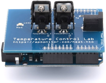
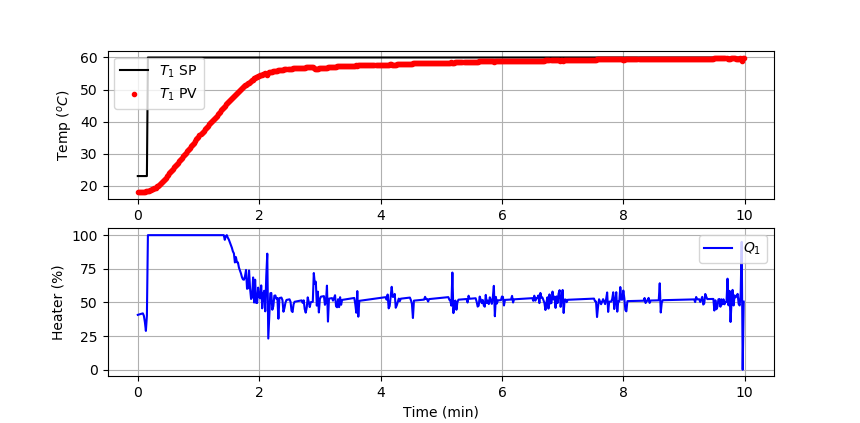
Objective: Implement a discrete PID controller and test the performance with a setpoint change from 23^oC to 60^oC. Use the IMC aggressive tuning correlation.

A PID controller is an equation that adjusts the controller output, `Q(t)`. It is a calculation of the difference between the setpoint `T_{SP}` and process variable `T_{PV}`. The adjustable parameters are the controller gain, `K_c`, and controller reset time or integral time constant, `\tau_I`. A large gain or small integral time constant produces a controller that reacts aggresively to a difference between the measured PV and target SP.

$$e(t) = T_{SP}-T_{PV}$$

$$Q(t) = Q_{bias} + K_c \, e(t) + \frac{K_c}{\tau_I}\int_0^t e(t) dt - K_c \tau_D \frac{d\left(T_{PV}\right)}{dt}$$

The `Q_{bias}` term is a constant that is typically set to the value of `Q(t)` when the controller is first switched from manual to automatic mode. The deviation variable for the heater is the change in value `Q'(t) = Q(t) - Q_{bias}`. For the TCLab, `Q_{bias}`=0 because the TCLab starts with the heater off. The `Q_{bias}` gives bumpless transfer if the error is zero when the controller is turned on. The continuous integral is approximated in a discrete form as a summation of the error multiplied by the sample time.

$$\frac{K_c}{\tau_I}\int_0^t e(t) dt \approx \frac{K_c}{\tau_I} \sum_{i=1}^{n_t} e_i(t)\Delta t$$

Likewise, the derivative term is a finite difference approximation. A common method uses the difference between the current and prior values of the PV to get the current slope.

$$\frac{d\left(T_{PV}\right)}{dt} \approx \frac{T_{PV,n_t}-T_{PV,n_t-1}}{\Delta t}$$

One potential problem with this form is that measurement noise is amplified and can cause controller output fluctuations. One way to reduce this is to use a first order filter or linear regression from the prior n time points. The PID equation in discrete form is the following:

$$Q(t) = Q_{bias} + K_c \,e(t) + \frac{K_c}{\tau_I} \sum_{i=1}^{n_t} e_i(t)\Delta t - K_c \tau_D \frac{T_{PV,n_t}-T_{PV,n_t-1}}{\Delta t}$$

Python PID Function

This equation can be implemented in Python as a function with inputs:

• sp = setpoint
• pv = current temperature
• pv_last = prior temperature
• ierr = integral error
• dt = time increment between measurements

and outputs:

• op = output of the PID controller
• P = proportional contribution
• I = integral contribution
• D = derivative contribution

The output Integral contribution (I) must be fed back in as an input to the function each successive call. The tuning parameters Kc, tauI, and tauD are defined as global variables or they could also be switched to function inputs.

IMC Aggressive Tuning

Use an IMC aggressive tuning correlation with FOPDT parameters (`K_c`, `\tau_p`, `\theta_p`) determined from the TCLab graphical fitting or TCLab regression exercises.

$$\mathrm{Aggressive\,Tuning:} \quad \tau_c = \max \left( 0.1 \tau_p, 0.8 \theta_p \right)$$

$$K_c = \frac{1}{K_p}\frac{\tau_p+0.5\theta_p}{\left( \tau_c + 0.5\theta_p \right)} \quad \quad \tau_I = \tau_p + 0.5 \theta_p \quad \quad \tau_D = \frac{\tau_p\theta_p}{2\tau_p + \theta_p}$$

Fill in the values of `K_c`, `\tau_I`, `\tau_D`, and the PID equation in the code below. Use anti-reset windup to prevent the integral from accumulating when the heater is saturated at 0% or 100%. Show a plot of the SP (temperature setpoint), PV (measured temperature), and OP (heater value) and report the integral absolute error between the setpoint and measured temperature.

PID Control Starting Script

See additional information on PID controllers.

Solution

import numpy as np
import matplotlib.pyplot as plt
import tclab
import time

# process model
Kp = 0.9
taup = 175.0
thetap = 15.0

# -----------------------------
# Calculate Kc,tauI,tauD (IMC Aggressive)
# -----------------------------
tauc = max(0.1*taup,0.8*thetap)
Kc = (1/Kp)*(taup+0.5*thetap)/(tauc+0.5*thetap)
tauI = taup + 0.5*thetap
tauD = taup*thetap / (2*taup+thetap)

print('Kc: ' + str(Kc))
print('tauI: ' + str(tauI))
print('tauD: ' + str(tauD))

#------------------------
# PID Controller Function
#------------------------
# sp = setpoint
# pv = current temperature
# pv_last = prior temperature
# ierr = integral error
# dt = time increment between measurements
# outputs ---------------
# op = output of the PID controller
# P = proportional contribution
# I = integral contribution
# D = derivative contribution
def pid(sp,pv,pv_last,ierr,dt):
    # Parameters in terms of PID coefficients
    KP = Kc
    KI = Kc/tauI
    KD = Kc*tauD
    # ubias for controller (initial heater)
    op0 = 0
    # upper and lower bounds on heater level
    ophi = 100
    oplo = 0
    # calculate the error
    error = sp-pv
    # calculate the integral error
    ierr = ierr + KI * error * dt
    # calculate the measurement derivative
    dpv = (pv - pv_last) / dt
    # calculate the PID output
    P = KP * error
    I = ierr
    D = -KD * dpv
    op = op0 + P + I + D
    # implement anti-reset windup
    if op < oplo or op > ophi:
        I = I - KI * error * dt
        # clip output
        op = max(oplo,min(ophi,op))
    # return the controller output and PID terms
    return [op,P,I,D]

n = 600  # Number of second time points (10 min)
tm = np.linspace(0,n-1,n) # Time values
lab = tclab.TCLab()
T1 = np.zeros(n)
Q1 = np.zeros(n)
# step setpoint from 23.0 to 60.0 degC
SP1 = np.ones(n)*23.0
SP1[10:] = 60.0
Q1_bias = 0.0
ierr = 0.0
for i in range(n):
    # record measurement
    T1[i] = lab.T1

    # --------------------------------------------------
    # call PID controller function to change Q1[i]
    # --------------------------------------------------
    [Q1[i],P,ierr,D] = pid(SP1[i],T1[i],T1[max(0,i-1)],ierr,1.0)

    lab.Q1(Q1[i])
    if i%20==0:
        print(' Heater,   Temp,  Setpoint')
    print(f'{Q1[i]:7.2f},{T1[i]:7.2f},{SP1[i]:7.2f}')
    # wait for 1 sec
    time.sleep(1)
lab.close()
# Save data file
data = np.vstack((tm,Q1,T1,SP1)).T
np.savetxt('PID_control.csv',data,delimiter=',',\
           header='Time,Q1,T1,SP1',comments='')

# Create Figure
plt.figure(figsize=(10,7))
ax = plt.subplot(2,1,1)
ax.grid()
plt.plot(tm/60.0,SP1,'k-',label=r'$T_1$ SP')
plt.plot(tm/60.0,T1,'r.',label=r'$T_1$ PV')
plt.ylabel(r'Temp ($^oC$)')
plt.legend(loc=2)
ax = plt.subplot(2,1,2)
ax.grid()
plt.plot(tm/60.0,Q1,'b-',label=r'$Q_1$')
plt.ylabel(r'Heater (%)')
plt.xlabel('Time (min)')
plt.legend(loc=1)
plt.savefig('PID_Control.png')
plt.show()

[$[Get Code]]

Generative AI Learning

Use these prompts to test your understanding after completing the exercise. Direct the AI - do not let it do the exercise for you.

App: Compare PID forms with the TCLab Control Studio - run velocity-form PID Types A, B, and C on the digital twin with the same tuning, observe how each handles setpoint changes and noise, and export the CSV for your report.

What to Turn In

Submit a short report (PDF, 1-2 pages) that curates your results into a demonstration of what you learned. You may use Generative AI to help write the report, but you must guide it to the correct visualizations, justifications, and assumptions. Answer these questions:

1. Include setpoint response plots for PI vs PID with the same Kc and tau-I. What did adding derivative change (overshoot, settling time, heater activity)?
2. From the app: how do PID Types A, B, and C differ in response to a setpoint step, and why (which terms act on error vs measurement)?
3. Would you enable derivative action on this loop in practice? Justify with your data and noise observations.
4. From the diagnostic prompt: what was the root cause and which fix did you validate?