TCLab Cascade Control
 |  | |  |  |  |
|---|
Objective: Design, tune, and test a cascade controller for the temperature control lab.
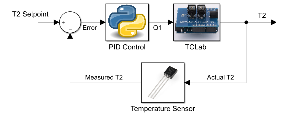
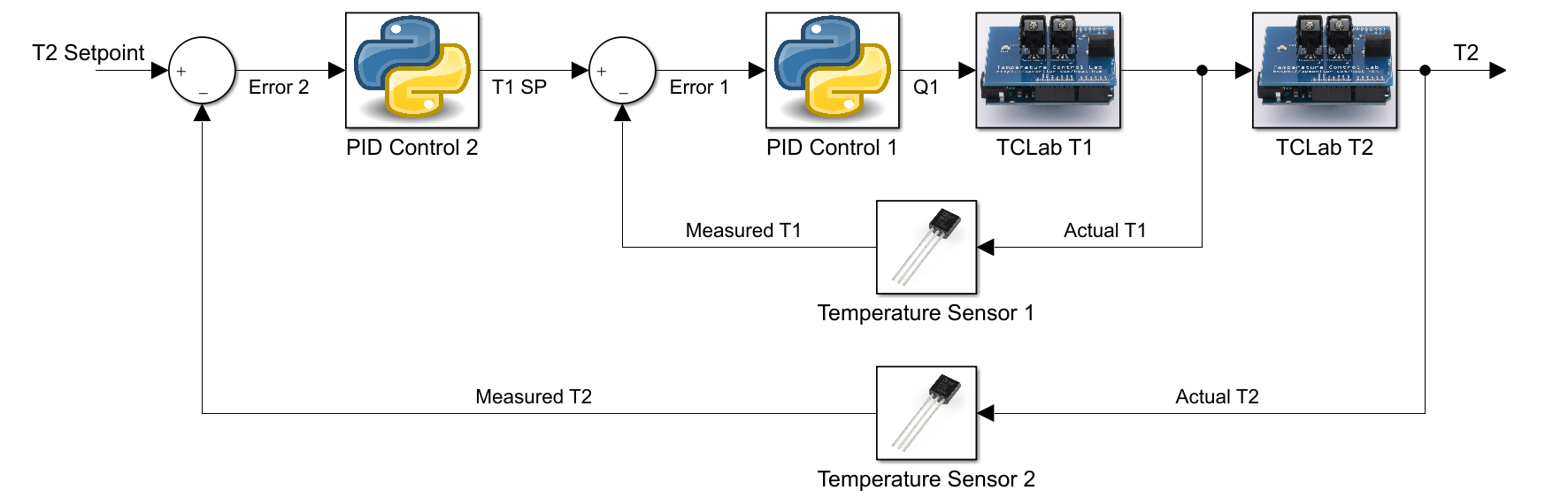
Design a cascade controller by labeling a block diagram that includes the inner and outer control loops. The inner loop is a T1 controller that has Q1 as the controller output. The outer loop is a T2 controller that has T1,SP as the controller output.
Tune the cascade controller with the TCLab to meet a temperature 2 (T2) target set point by adjusting heater 1 (Q1). Minimize the integral absolute error (IAE) while staying below 85oC for temperature 1 (T1). Compare the cascade control performance with a standard PI controller.


%matplotlib inline
import matplotlib.pyplot as plt
from scipy.integrate import odeint
import ipywidgets as wg
from IPython.display import display
n = 1201 # time points to plot
tf = 1200.0 # final time
# TCLab Second-Order
Kp = 0.8473
Kd = 0.3
taus = 51.08
zeta = 1.581
thetap = 0.0
def process(z,t,u):
x1,y1,x2,y2 = z
dx1dt = (1.0/(taus**2)) * (-2.0*zeta*taus*x1-(y1-23.0) + Kp*u + Kd*(y2-y1))
dy1dt = x1
dx2dt = (1.0/(taus**2)) * (-2.0*zeta*taus*x2-(y2-23.0) + Kd*(y1-y2))
dy2dt = x2
return [dx1dt,dy1dt,dx2dt,dy2dt]
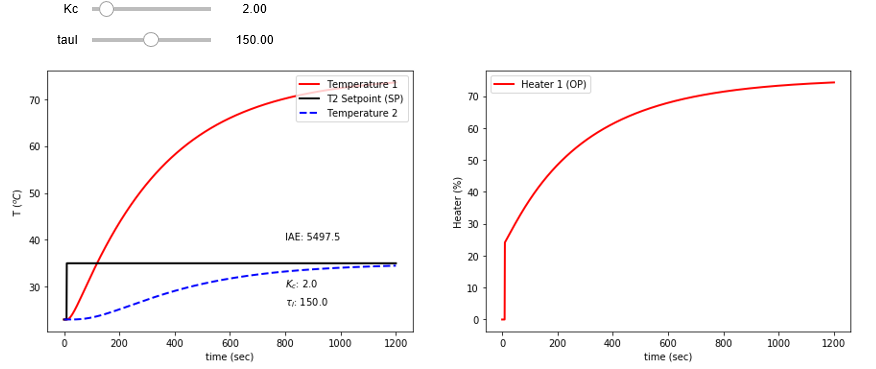
def pidPlot(Kc,tauI):
t = np.linspace(0,tf,n) # create time vector
P = np.zeros(n) # initialize proportional term
I = np.zeros(n) # initialize integral term
e = np.zeros(n) # initialize error
ie = np.zeros(n) # initialize integral error
OP = np.zeros(n) # initialize controller output
PV1 = np.ones(n)*23.0 # initialize process variable
PV2 = np.ones(n)*23.0 # initialize process variable
SP2 = np.ones(n)*23.0 # initialize setpoint
SP2[10:] = 35.0 # step up
z0 = [0,23.0,0,23.0] # initial condition
# loop through all time steps
for i in range(1,n):
# simulate process for one time step
ts = [t[i-1],t[i]] # time interval
z = odeint(process,z0,ts,args=(OP[max(0,i-1-int(thetap))],))
z0 = z[1] # record new initial condition
# calculate new OP with PID
PV1[i] = z0[1] # record PV 1
PV2[i] = z0[3] # record PV 2
e[i] = SP2[i] - PV2[i] # calculate error = SP - PV
ie[i] = e[i] + ie[i-1]
dt = t[i] - t[i-1] # calculate time step
P[i] = Kc * e[i] # calculate proportional term
I[i] = Kc/tauI * ie[i]
OP[i] = min(100,max(0,P[i]+I[i])) # calculate new controller output
if OP[i]==100 or OP[i]==0:
ie[i] = ie[i-1] # anti-windup
# plot PID response
plt.figure(1,figsize=(15,5))
plt.subplot(1,2,1)
plt.plot(t,PV1,'r-',linewidth=2,label='Temperature 1')
plt.plot(t,SP2,'k-',linewidth=2,label='T2 Setpoint (SP)')
plt.plot(t,PV2,'b--',linewidth=2,label='Temperature 2')
plt.ylabel(r'T $(^oC)$')
plt.text(800,30,r'$K_c$: ' + str(np.round(Kc,1)))
plt.text(800,26,r'$\tau_I$: ' + str(np.round(tauI,1)))
plt.text(800,40,r'IAE: ' + str(np.round(np.sum(np.abs(e)),1)))
plt.legend(loc=1)
plt.xlabel('time (sec)')
plt.subplot(1,2,2)
plt.plot(t,OP,'r-',linewidth=2,label='Heater 1 (OP)')
plt.ylabel('Heater (%)')
plt.legend(loc='best')
plt.xlabel('time (sec)')
Kc_slide = wg.FloatSlider(value=2.0,min=1.0,max=10.0,step=1.0)
tauI_slide = wg.FloatSlider(value=150.0,min=5.0,max=300.0,step=5.0)
wg.interact(pidPlot, Kc=Kc_slide, tauI=tauI_slide)
print('PI Control: Adjust Kc and tauI')
%matplotlib inline
import matplotlib.pyplot as plt
from scipy.integrate import odeint
import ipywidgets as wg
from IPython.display import display
n = 1201 # time points to plot
tf = 1200.0 # final time
# TCLab Second-Order
Kp = 0.8473
Kd = 0.3
taus = 51.08
zeta = 1.581
thetap = 0.0
def process(z,t,u):
x1,y1,x2,y2 = z
dx1dt = (1.0/(taus**2)) * (-2.0*zeta*taus*x1-(y1-23.0) + Kp*u + Kd*(y2-y1))
dy1dt = x1
dx2dt = (1.0/(taus**2)) * (-2.0*zeta*taus*x2-(y2-23.0) + Kd*(y1-y2))
dy2dt = x2
return [dx1dt,dy1dt,dx2dt,dy2dt]
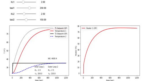
def pidPlot(Kc1,tauI1,Kc2,tauI2):
t = np.linspace(0,tf,n) # create time vector
P1 = np.zeros(n) # initialize proportional term
I1 = np.zeros(n) # initialize integral term
P2 = np.zeros(n) # initialize proportional term
I2 = np.zeros(n) # initialize integral term
e1 = np.zeros(n) # initialize error
ie1 = np.zeros(n) # initialize integral error
e2 = np.zeros(n) # initialize error
ie2 = np.zeros(n) # initialize integral error
OP = np.zeros(n) # initialize controller output
PV1 = np.ones(n)*23.0 # initialize process variable
PV2 = np.ones(n)*23.0 # initialize process variable
SP1 = np.ones(n)*23.0 # initialize setpoint
SP2 = np.ones(n)*23.0 # initialize setpoint
SP2[10:] = 35.0 # step up
z0 = [0,23.0,0,23.0] # initial condition
iae = 0.0
# loop through all time steps
for i in range(1,n):
# simulate process for one time step
ts = [t[i-1],t[i]] # time interval
z = odeint(process,z0,ts,args=(OP[max(0,i-1-int(thetap))],))
z0 = z[1] # record new initial condition
dt = t[i] - t[i-1] # calculate time step
# outer loop
PV2[i] = z0[3] # record PV 2
e2[i] = SP2[i] - PV2[i] # calculate error = SP - PV
ie2[i] = e2[i]*dt + ie2[i-1]
P2[i] = Kc2 * e2[i] # calculate proportional term
I2[i] = Kc2/tauI2 * ie2[i]
SP1[i] = min(85,max(23,P2[i]+I2[i])) # calculate new controller output
if SP1[i]==85 or SP1[i]==23:
ie2[i] = ie2[i-1] # anti-windup
# inner loop
PV1[i] = z0[1] # record PV 1
e1[i] = SP1[i] - PV1[i] # calculate error = SP - PV
ie1[i] = e1[i]*dt + ie1[i-1]
P1[i] = Kc1 * e1[i] # calculate proportional term
I1[i] = Kc1/tauI1 * ie1[i]
OP[i] = min(100,max(0,P1[i]+I1[i])) # calculate new controller output
if OP[i]==100 or OP[i]==0:
ie1[i] = ie1[i-1] # anti-windup
# plot PID response
plt.figure(1,figsize=(15,5))
plt.subplot(1,2,1)
plt.plot(t,SP1,'k:',linewidth=2,label='T1 Setpoint (SP)')
plt.plot(t,PV1,'r-',linewidth=2,label='Temperature 1')
plt.plot(t,SP2,'k-',linewidth=2,label='T2 Setpoint (SP)')
plt.plot(t,PV2,'b--',linewidth=2,label='Temperature 2')
plt.ylabel(r'T $(^oC)$')
plt.text(500,30,'Inner Loop 1')
plt.text(500,26,r'$K_{c1}$: ' + str(np.round(Kc1,1)))
plt.text(500,22,r'$\tau_{I1}$: ' + str(np.round(tauI1,1)))
plt.text(800,30,'Outer Loop 2')
plt.text(800,26,r'$K_{c2}$: ' + str(np.round(Kc2,1)))
plt.text(800,22,r'$\tau_{I2}$: ' + str(np.round(tauI2,1)))
plt.text(800,40,r'IAE: ' + str(np.round(np.sum(np.abs(e2)),1)))
plt.legend(loc=1)
plt.xlabel('time (sec)')
plt.subplot(1,2,2)
plt.plot(t,OP,'r-',linewidth=2,label='Heater 1 (OP)')
plt.ylabel('Heater (%)')
plt.legend(loc='best')
plt.xlabel('time (sec)')
Kc1_slide = wg.FloatSlider(value=2.0,min=1.0,max=10.0,step=0.5)
tauI1_slide = wg.FloatSlider(value=200.0,min=5.0,max=300.0,step=5.0)
Kc2_slide = wg.FloatSlider(value=3.0,min=2.0,max=10.0,step=0.5)
tauI2_slide = wg.FloatSlider(value=150.0,min=5.0,max=300.0,step=5.0)
wg.interact(pidPlot, Kc1=Kc1_slide, tauI1=tauI1_slide, \
Kc2=Kc2_slide, tauI2=tauI2_slide)
print('PI Cascade Control: Adjust Kc1, Kc2, tauI1, tauI2')
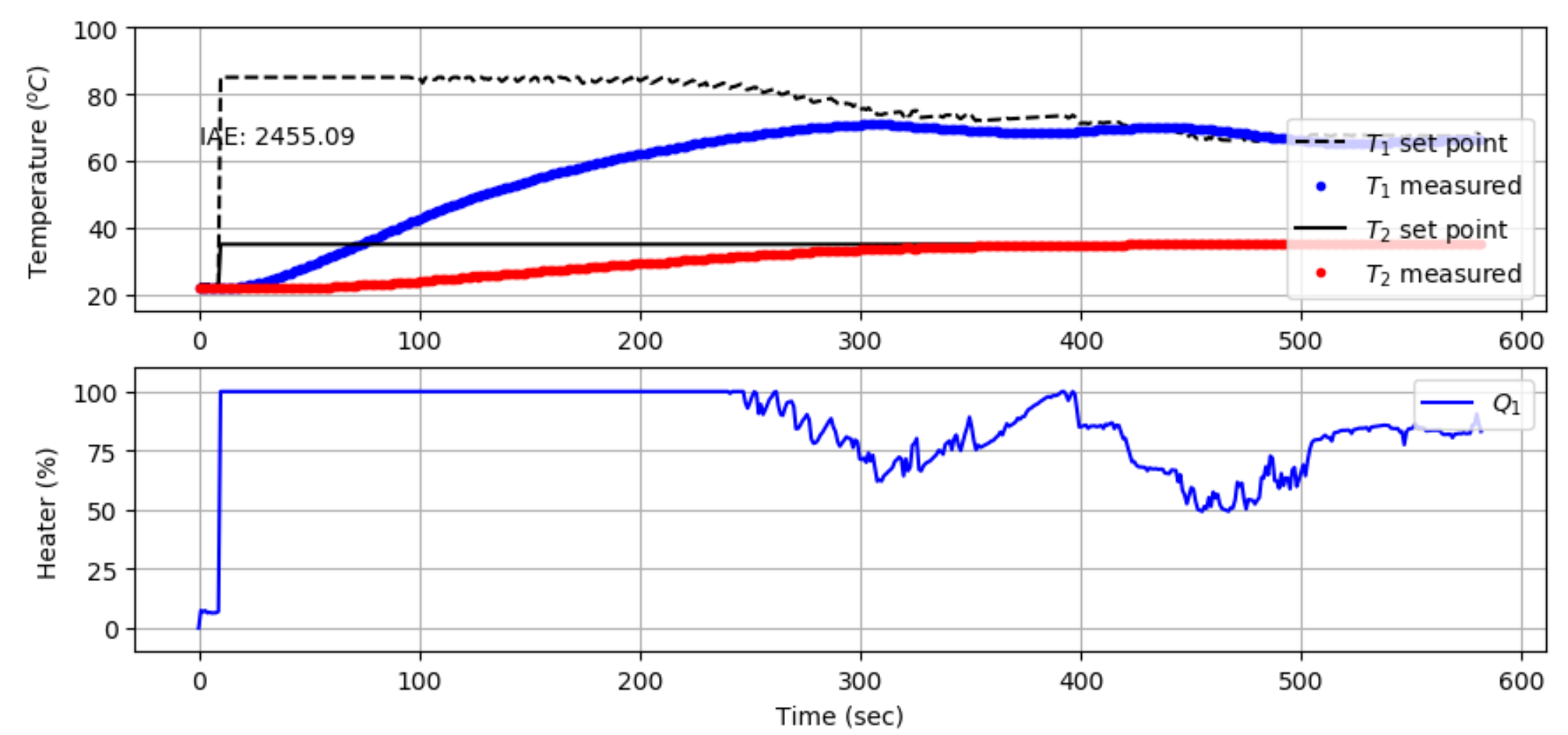
Test the cascade control on the TCLab. Discuss any differences between the simulated and measured values.
import numpy as np
import time
import matplotlib.pyplot as plt
from scipy.integrate import odeint
#-----------------------------------------
# PID controller performance for the TCLab
#-----------------------------------------
# PID Parameters
Kc1 = 5.0
tauI1 = 50.0 # sec
Kc2 = 3.0
tauI2 = 100.0 # sec
# Animate Plot?
animate = True
if animate:
try:
from IPython import get_ipython
from IPython.display import display,clear_output
get_ipython().run_line_magic('matplotlib', 'inline')
ipython = True
print('IPython Notebook')
except:
ipython = False
print('Not IPython Notebook')
#-----------------------------------------
# Cascade PID Controller
#-----------------------------------------
# inputs ---------------------------------
# sp = setpoint
# pv = current temperature
# pv_last = prior temperature
# ierr = integral error
# dt = time increment between measurements
# outputs --------------------------------
# op = output of the PID controller
# P = proportional contribution
# I = integral contribution
# D = derivative contribution
def pid(sp,pv,pv_last,ierr,dt,d,cid):
# Parameters in terms of PID coefficients
if cid==1:
# controller 1
KP = Kc1
KI = Kc1/tauI1
ophi = 100
oplo = 0
else:
# controller 2
KP = Kc2
KI = Kc2/tauI2
ophi = 85
oplo = 23
# ubias for controller (initial heater)
op0 = 0
# calculate the error
error = sp-pv
# calculate the integral error
ierr = ierr + KI * error * dt
# calculate the measurement derivative
dpv = (pv - pv_last) / dt
# calculate the PID output
P = KP * error
I = ierr
op = op0 + P + I
# implement anti-reset windup
if op < oplo or op > ophi:
I = I - KI * error * dt
# clip output
op = max(oplo,min(ophi,op))
# return the controller output and PID terms
return [op,P,I]
# save txt file with data and set point
# t = time
# u1,u2 = heaters
# y1,y2 = tempeatures
# sp1,sp2 = setpoints
def save_txt(t, u1, u2, y1, y2, sp1, sp2):
data = np.vstack((t, u1, u2, y1, y2, sp1, sp2)) # vertical stack
data = data.T # transpose data
top = ('Time,Q1,Q2,T1,T2,TSP1,TSP2')
np.savetxt('validate.txt', data, delimiter=',',\
header=top, comments='')
# Connect to Arduino
a = tclab.TCLab()
# Wait until temperature is below 25 degC
print('Check that temperatures are < 25 degC before starting')
i = 0
while a.T1>=25.0 or a.T2>=25.0:
print(f'Time: {i} T1: {a.T1} T2: {a.T2}')
i += 10
time.sleep(10)
# Turn LED on
print('LED On')
a.LED(100)
# Run time in minutes
run_time = 15.0
# Number of cycles
loops = int(60.0*run_time)
tm = np.zeros(loops)
# Heater set point steps
Tsp1 = np.ones(loops) * a.T1
Tsp2 = np.ones(loops) * a.T2
Tsp2[10:] = 35.0 # step up
T1 = np.ones(loops) * a.T1 # measured T (degC)
T2 = np.ones(loops) * a.T2 # measured T (degC)
# impulse tests (0 - 100%)
Q1 = np.ones(loops) * 0.0
Q2 = np.ones(loops) * 0.0
if not animate:
print('Running Main Loop. Ctrl-C to end.')
print(' Time SP1 PV1 Q1 SP2 PV2 Q2 IAE')
print(('{:6.1f} {:6.2f} {:6.2f} ' + \
'{:6.2f} {:6.2f} {:6.2f} {:6.2f} {:6.2f}').format( \
tm[0],Tsp1[0],T1[0],Q1[0],Tsp2[0],T2[0],Q2[0],0.0))
# Main Loop
start_time = time.time()
prev_time = start_time
dt_error = 0.0
# Integral error
ierr1 = 0.0
ierr2 = 0.0
# Integral absolute error
iae = 0.0
if not ipython:
plt.figure(figsize=(10,7))
plt.ion()
plt.show()
try:
for i in range(1,loops):
# Sleep time
sleep_max = 1.0
sleep = sleep_max - (time.time() - prev_time) - dt_error
if sleep>=1e-4:
time.sleep(sleep-1e-4)
else:
print('exceeded max cycle time by ' + str(abs(sleep)) + ' sec')
time.sleep(1e-4)
# Record time and change in time
t = time.time()
dt = t - prev_time
if (sleep>=1e-4):
dt_error = dt-sleep_max+0.009
else:
dt_error = 0.0
prev_time = t
tm[i] = t - start_time
# Read temperatures in Kelvin
T1[i] = a.T1
T2[i] = a.T2
# Disturbances
d1 = T1[i] - 23.0
d2 = T2[i] - 23.0
# Integral absolute error
iae += np.abs(np.abs(Tsp2[i]-T2[i]))
# Calculate PID output
[Tsp1[i],P,ierr2] = pid(Tsp2[i],T2[i],T2[i-1],ierr2,dt,d1,2)
[Q1[i],P,ierr1] = pid(Tsp1[i],T1[i],T1[i-1],ierr1,dt,d2,1)
# Write output (0-100)
a.Q1(Q1[i])
a.Q2(0)
if not animate:
# Print line of data
print(('{:6.1f} {:6.2f} {:6.2f} ' + \
'{:6.2f} {:6.2f} {:6.2f} {:6.2f} {:6.2f}').format( \
tm[i],Tsp1[i],T1[i],Q1[i],Tsp2[i],T2[i],Q2[i],iae))
else:
if ipython:
plt.figure(figsize=(10,7))
else:
plt.clf()
# Update plot
ax=plt.subplot(2,1,1)
ax.grid()
plt.plot(tm[0:i],Tsp1[0:i],'k--',label=r'$T_1$ set point')
plt.plot(tm[0:i],T1[0:i],'r.',label=r'$T_1$ measured')
plt.plot(tm[0:i],Tsp2[0:i],'k-',label=r'$T_2$ set point')
plt.plot(tm[0:i],T2[0:i],'b.',label=r'$T_2$ measured')
plt.ylabel(r'Temperature ($^oC$)')
plt.text(0,65,'IAE: ' + str(np.round(iae,2)))
plt.legend(loc=4)
plt.ylim([15,100])
ax=plt.subplot(2,1,2)
ax.grid()
plt.plot(tm[0:i],Q1[0:i],'b-',label=r'$Q_1$')
plt.ylim([-10,110])
plt.ylabel('Heater (%)')
plt.legend(loc=1)
plt.xlabel('Time (sec)')
if ipython:
clear_output(wait=True)
display(plt.gcf())
else:
plt.draw()
plt.pause(0.05)
# Turn off heaters
a.Q1(0)
a.Q2(0)
a.close()
# Save text file
save_txt(tm,Q1,Q2,T1,T2,Tsp1,Tsp2)
# Save Plot
if not animate:
plt.figure(figsize=(10,7))
ax=plt.subplot(2,1,1)
ax.grid()
plt.plot(tm,Tsp1,'k--',label=r'$T_1$ set point')
plt.plot(tm,T1,'r.',label=r'$T_1$ measured')
plt.plot(tm,Tsp2,'k-',label=r'$T_2$ set point')
plt.plot(tm,T2,'b.',label=r'$T_2$ measured')
plt.ylabel(r'Temperature ($^oC$)')
plt.text(0,65,'IAE: ' + str(np.round(iae,2)))
plt.legend(loc=4)
ax=plt.subplot(2,1,2)
ax.grid()
plt.plot(tm,Q1,'b-',label=r'$Q_1$')
plt.ylabel('Heater (%)')
plt.legend(loc=1)
plt.xlabel('Time (sec)')
plt.savefig('PID_Control.png')
# Allow user to end loop with Ctrl-C
except KeyboardInterrupt:
# Disconnect from Arduino
a.Q1(0)
a.Q2(0)
print('Shutting down')
a.close()
save_txt(tm[0:i],Q1[0:i],Q2[0:i],T1[0:i],T2[0:i],Tsp1[0:i],Tsp2[0:i])
plt.savefig('PID_Control.png')
# Make sure serial connection closes with an error
except:
# Disconnect from Arduino
a.Q1(0)
a.Q2(0)
print('Error: Shutting down')
a.close()
save_txt(tm[0:i],Q1[0:i],Q2[0:i],T1[0:i],T2[0:i],Tsp1[0:i],Tsp2[0:i])
plt.savefig('PID_Control.png')
raise
print('Cascade control test complete')
Solution
Design: A standard feedback control system includes only one measurement (T2) and one actuator (Q1) that is adjusted to meet the setpoint (T2,SP).
By adding the second measurement (T1) and another PID controller with (T1,SP) as the inner loop, cascade control is implemented.
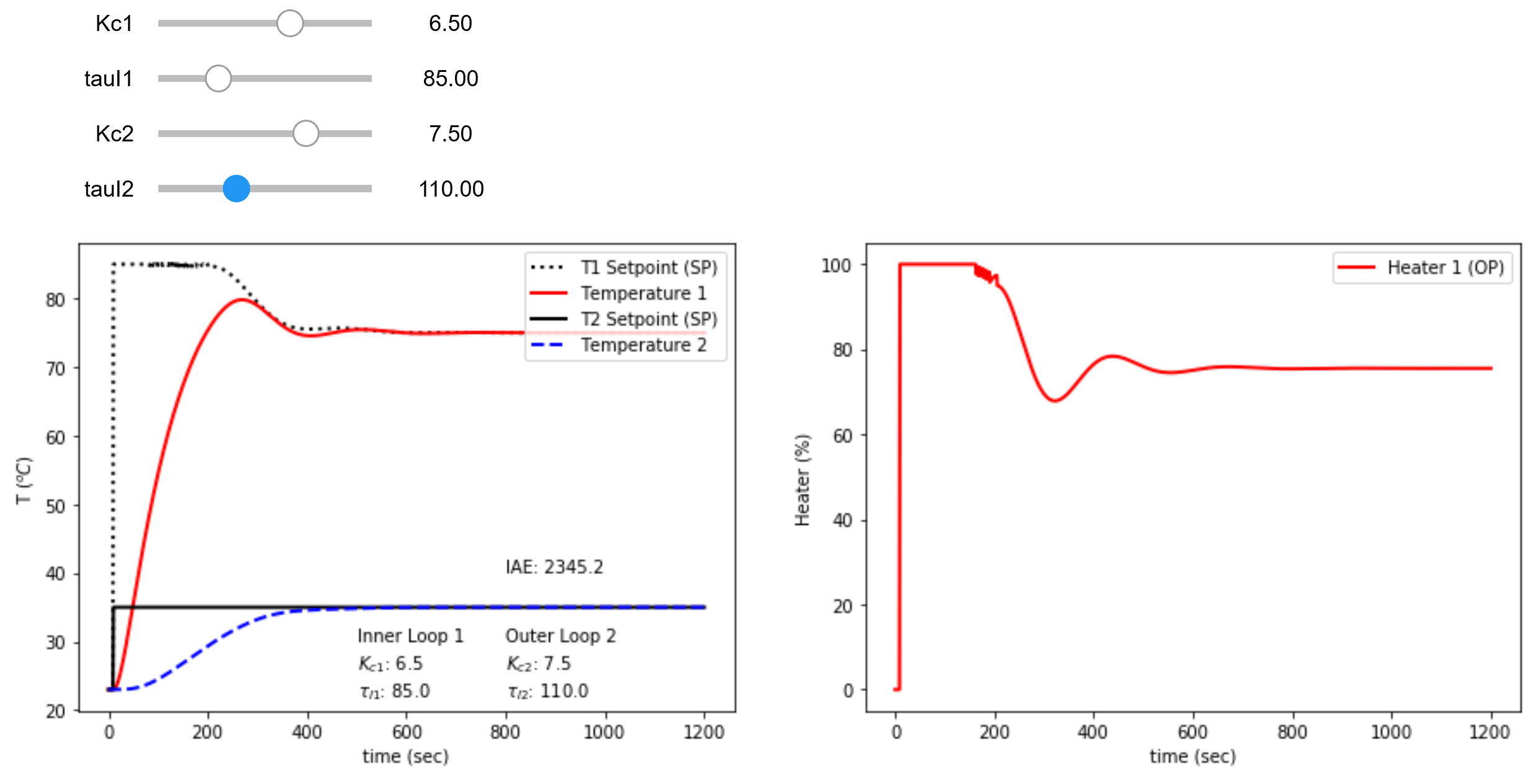
Tune the cascade controller involves minimizing the integral absolute error (IAE) while staying below 85oC for temperature 1 (T1). The controller output (T1,SP) from the outer controller (T2) is set to 85oC to avoid overshooting the upper limit constraint. The anticipated cascade performance is IAE = 2345.2.
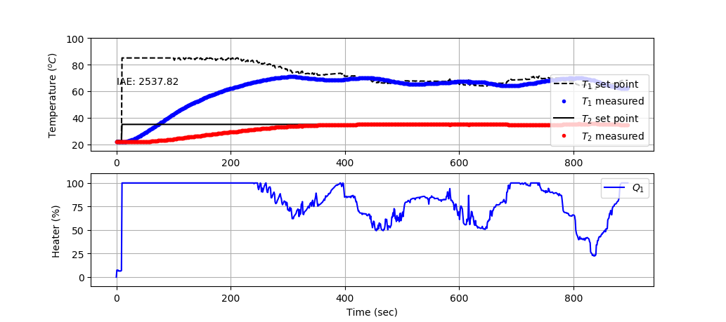
Test: The 15 minute test gives a larger IAE by about 8% ((2537.8-2345.2)/2345.2) than predicted because of unmodeled disturbances that are not included in the simulation. This is evident from the Q1 adjustments even after T2 reaches the setpoint.
Kc1 = 6.5
tauI1 = 85.0 # sec
Kc2 = 7.5
tauI2 = 110.0 # sec
What to Turn In
- Item 1: Labeled cascade block diagram showing inner (Q₁ to T₁) and outer (`T_{1,SP}` to T₂) loops with all signals labeled.
- Item 2: Final tuning summary: Kc₁, `\tau_{I1}` (inner loop) and Kc₂, `\tau_{I2}` (outer loop), plus a short note on how you ensured T₁ ≤ 85 °C (e.g., setpoint/OP clipping, anti-windup).
- Item 3: Simulation results for standard PI vs. cascade: plots of T₁, T₂, setpoints, and Q₁ over 1200s with IAE values reported for both.
- Item 4: TCLab test: plot comparing measured vs. simulated responses for cascade control. Report measured IAE and comment on any offsets/disturbances.
- Item 5: Brief comparison and conclusions: when cascade outperforms single-loop PI for this plant and why (inner-loop bandwidth, disturbance pathways), with your recommended gains.