Energy Balance Parameter Estimation
The objective of this activity is to fit the physics-based predictions to the data as well as fit a first-order plus dead-time (FOPDT) model to the data. In both cases, select parameters are adjusted to minimize an objective function such as a sum of squared errors between the model predicted values and the measured values. Test the temperature response of the Arduino device by introducing a step in the heater.
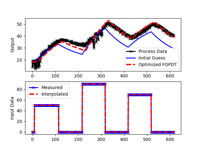
Fit FOPDT Model with Optimization
Determine the parameters of an FOPDT model that best match the dynamic temperature data including `K_p`, `\tau_p`, and `\theta_p`. A second order (SOPDT) can also be fit to investigate whether a higher order model is more accurate.
import matplotlib.pyplot as plt
from scipy.integrate import odeint
from scipy.optimize import minimize
from scipy.interpolate import interp1d
# Import CSV data file
# Column 1 = time (t)
# Column 2 = input (u)
# Column 3 = output (yp)
data = np.loadtxt('data.txt',delimiter=',',skiprows=1)
u0 = data[0,1]
yp0 = data[0,3]
t = data[:,0].T - data[0,0]
u = data[:,1].T
yp = data[:,3].T
# specify number of steps
ns = len(t)
delta_t = t[1]-t[0]
# create linear interpolation of the u data versus time
uf = interp1d(t,u)
# define first-order plus dead-time approximation
def fopdt(y,t,uf,Km,taum,thetam):
# arguments
# y = output
# t = time
# uf = input linear function (for time shift)
# Km = model gain
# taum = model time constant
# thetam = model time constant
# time-shift u
try:
if (t-thetam) <= 0:
um = uf(0.0)
else:
um = uf(t-thetam)
except:
#print('Error with time extrapolation: ' + str(t))
um = u0
# calculate derivative
dydt = (-(y-yp0) + Km * (um-u0))/taum
return dydt
# simulate FOPDT model with x=[Km,taum,thetam]
def sim_model(x):
# input arguments
Km = x[0]
taum = x[1]
thetam = x[2]
# storage for model values
ym = np.zeros(ns) # model
# initial condition
ym[0] = yp0
# loop through time steps
for i in range(0,ns-1):
ts = [t[i],t[i+1]]
y1 = odeint(fopdt,ym[i],ts,args=(uf,Km,taum,thetam))
ym[i+1] = y1[-1]
return ym
# define objective
def objective(x):
# simulate model
ym = sim_model(x)
# calculate objective
obj = 0.0
for i in range(len(ym)):
obj = obj + (ym[i]-yp[i])**2
# return result
return obj
# initial guesses
x0 = np.zeros(3)
x0[0] = 0.5 # Km
x0[1] = 120.0 # taum
x0[2] = 0.0 # thetam
# show initial objective
print('Initial SSE Objective: ' + str(objective(x0)))
# optimize Km, taum, thetam
solution = minimize(objective,x0)
# Another way to solve: with bounds on variables
#bnds = ((0.4, 0.6), (1.0, 10.0), (0.0, 30.0))
#solution = minimize(objective,x0,bounds=bnds,method='SLSQP')
x = solution.x
# show final objective
print('Final SSE Objective: ' + str(objective(x)))
print('Kp: ' + str(x[0]))
print('taup: ' + str(x[1]))
print('thetap: ' + str(x[2]))
# calculate model with updated parameters
ym1 = sim_model(x0)
ym2 = sim_model(x)
# plot results
plt.figure()
plt.subplot(2,1,1)
plt.plot(t,yp,'kx-',linewidth=2,label='Process Data')
plt.plot(t,ym1,'b-',linewidth=2,label='Initial Guess')
plt.plot(t,ym2,'r--',linewidth=3,label='Optimized FOPDT')
plt.ylabel('Output')
plt.legend(loc='best')
plt.subplot(2,1,2)
plt.plot(t,u,'bx-',linewidth=2)
plt.plot(t,uf(t),'r--',linewidth=3)
plt.legend(['Measured','Interpolated'],loc='best')
plt.ylabel('Input Data')
plt.savefig('fopdt_fit.png')
plt.show()
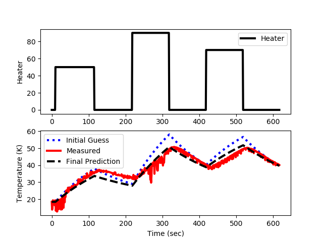
Fit Physics-Based Model with Optimization
The full energy balance includes convection and radiation terms.
$$m\,c_p\frac{dT}{dt} = U\,A\,\left(T_\infty-T\right) + \epsilon\,\sigma\,A\,\left(T_\infty^4-T^4\right) + \alpha Q$$
where `m` is the mass, `c_p` is the heat capacity, `T` is the temperature, `U` is the heat transfer coefficient, `A` is the area, `T_\infty` is the ambient temperature, `\epsilon=0.9` is the emissivity, `\sigma =` 5.67x10⁻⁸ `W/{m^2 K^4}` is the Stefan-Boltzmann constant, and `Q` is the percentage heater output. The parameter `\alpha` is a factor that relates heater output (0-100%) to power dissipated by the transistor in Watts.
Adjust the uncertain parameters such as `U` and `\alpha` from the modeling exercise to best match the dynamic data from the impulse response.
import matplotlib.pyplot as plt
from scipy.integrate import odeint
from scipy.optimize import minimize
# Import data file
# Column 1 = time (t)
# Column 2 = input (u)
# Column 3 = output (yp)
data = np.loadtxt('data.txt',delimiter=',',skiprows=1)
# initial conditions
Q0 = data[0,1]
Tmeas0 = data[0,3]
# extract data columns
t = data[:,0].T
Q = data[:,1].T
Tmeas = data[:,3].T
# specify number of steps
ns = len(t)
delta_t = t[1]-t[0]
Cp = 0.5 * 1000.0 # J/kg-K
A = 12.0 / 100.0**2 # Area in m^2
Ta = Tmeas0 # Ambient temperature (K)
# define energy balance model
def heat(x,t,Q,p):
# Adjustable Parameters
U = p[0] # starting at 10.0 W/m^2-K
alpha = p[1] # starting as 0.01 W / % heater
# Known Parameters
m = 4.0/1000.0 # kg
Cp = 0.5 * 1000.0 # J/kg-K
A = 12.0 / 100.0**2 # Area in m^2
eps = 0.9 # Emissivity
sigma = 5.67e-8 # Stefan-Boltzman
# Temperature State
T = x[0]
# Nonlinear Energy Balance
dTdt = (1.0/(m*Cp))*(U*A*(Ta-T) \
+ eps * sigma * A * (Ta**4 - T**4) \
+ alpha*Q)
return dTdt
def calc_T(p):
T = np.ones(len(t)) * Tmeas0
T0 = T[0]
for i in range(len(t)-1):
ts = [t[i],t[i+1]]
y = odeint(heat,T0,ts,args=(Q[i],p))
T0 = y[-1]
T[i+1] = T0
return T
# define objective
def objective(p):
# simulate model
Tp = calc_T(p)
# calculate objective
obj = 0.0
for i in range(len(Tmeas)):
obj = obj + ((Tp[i]-Tmeas[i])/Tmeas[i])**2
# return result
return obj
# Parameter initial guess
U = 10.0 # Heat transfer coefficient (W/m^2-K)
alpha = 0.01 # Heat gain (W/%)
p0 = [U,alpha]
# show initial objective
print('Initial SSE Objective: ' + str(objective(p0)))
# optimize parameters
# bounds on variables
bnds = ((2.0, 20.0),(0.005,0.02))
solution = minimize(objective,p0,method='SLSQP',bounds=bnds)
p = solution.x
# show final objective
print('Final SSE Objective: ' + str(objective(p)))
# optimized parameter values
U = p[0]
alpha = p[1]
print('U: ' + str(U))
print('alpha: ' + str(alpha))
# Known Parameters
m = 4.0/1000.0 # kg
Cp = 0.5 * 1000.0 # J/kg-K
A = 12.0 / 100.0**2 # Area in m^2
eps = 0.9 # Emissivity
sigma = 5.67e-8 # Stefan-Boltzman
T0 = Tmeas0
print('')
print('FOPDT Equivalent')
#dx/dt = (-1/taup) * x + (Kp/taup) * u
#dTdt = (1.0/(m*Cp))*(-h*A*(T-Ta) + Amp*mVi/1000.0)
dfdT = -(U*A-4.0*eps*sigma*A*T0**3)/(m*Cp)
dfdQ = alpha/(m*Cp)
taup = -1.0/dfdT
Kp = dfdQ * taup
print('Kp: ' + str(Kp))
print('taup: ' + str(taup))
# calculate model with updated parameters
T1 = calc_T(p0)
T2 = calc_T(p)
# Plot the results
plt.figure()
plt.subplot(2,1,1)
plt.plot(t,Q,'k-',linewidth=3)
plt.ylabel('Heater')
plt.legend(['Heater'],loc='best')
plt.subplot(2,1,2)
plt.plot(t,T1,'b:',linewidth=3,label='Initial Guess')
plt.plot(t,Tmeas,'r-',linewidth=3,label='Measured')
plt.plot(t,T2,'k--',linewidth=3,label='Final Prediction')
plt.ylabel('Temperature (K)')
plt.legend(loc='best')
plt.xlabel('Time (sec)')
plt.savefig('optimization.png')
plt.show()
Compare FOPDT and Linearized Model
A linearized version of the model can be used to compare an FOPDT model to the physics-based model. A linearized model is derived as:
$$m\,c_p\frac{dT}{dt} = f\left(T_\infty,T,V\right) \approx f \left(\bar T_\infty, \bar T, \bar V\right) \ldots \\ + \frac{\partial f}{\partial T_\infty}\bigg|_{\bar T_\infty,\bar T,\bar Q} \left(T_\infty-\bar T_\infty\right) \ldots \\ + \frac{\partial f}{\partial T}\bigg|_{\bar T_\infty,\bar T,\bar Q} \left(T-\bar T\right) \ldots \\ + \frac{\partial f}{\partial V}\bigg|_{\bar T_\infty,\bar T,\bar Q} \left(Q-\bar Q\right)$$
where
$$\frac{\partial f}{\partial T_\infty}\bigg|_{\bar T_\infty,\bar T,\bar Q} = U\,A\,\bar T_\infty + 4\epsilon\,\sigma\,A\,\bar T_\infty^3 = \beta$$
$$\frac{\partial f}{\partial T}\bigg|_{\bar T_\infty,\bar T,\bar Q} = -U\,A\,\bar T - 4\epsilon\,\sigma\,A\,\bar T^3 = \gamma$$
$$\frac{\partial f}{\partial Q}\bigg|_{\bar T_\infty,\bar T,\bar Q} = \alpha$$
The final linearized equation is further simplified by replacing the partial derivatives with constants `\beta`, `\gamma`, and `\alpha` that are evaluated at the steady state conditions `\bar T_\infty`, `\bar T`, and `\bar Q`.
$$m\,c_p\frac{dT}{dt} = \beta \left(T_\infty-\bar T_\infty\right) + \gamma \left(T-\bar T\right) + \alpha \left(Q-\bar Q\right)$$
This is placed into a time-constant form as by dividing by `gamma` and substituting the deviation variables `T\prime_\infty = T_\infty -\bar T_\infty`, `T\prime = T -\bar T`, and `Q\prime = Q -\bar Q`.
$$\frac{m\,c_p}{\gamma}\frac{dT^\prime}{dt} = \frac{\beta}{\gamma} T^\prime_\infty + T^\prime + \frac{\alpha}{\gamma} Q^\prime$$
Further simplification is possible with `\beta = -\gamma`.
$$\frac{m\,c_p}{\gamma}\frac{dT^\prime}{dt} = -T^\prime_\infty + T^\prime + \frac{\alpha}{\gamma} Q^\prime$$
Multiplying both sides by -1 puts the equation into a time constant form with new constants `\tau_P` and `K_p`.
$$\tau_P \frac{dT^\prime}{dt} = -T^\prime + T^\prime_\infty + K_p Q^\prime$$
$$K_P = -\frac{\alpha}{\gamma}$$ $$\tau_P = -\frac{m\,c_p}{\gamma}$$
This derivation does not include a time delay but the other parameters can be correlated to an empirical FOPDT fit of the data. Another way to fit the uncertain parameters such as overall heat transfer coefficient and `\alpha` is to use optimization methods. There is a script that demonstrates the use of optimization to minimize an objective function. The objective function is a minimization of the difference between the predicted and measured values.
Moving Horizon Estimation
Return to Temperature Control Lab Overview