Piecewise Linear
Piece-wise Linear Approximation
A piece-wise linear function is an approximation of a nonlinear relationship. For more nonlinear relationships, additional linear segments are added to refine the approximation.
As an example, the piecewise linear form is often used to approximate valve characterization (valve position (% open) to flow). This is a single input-single output function approximation.
In Situ Adaptive Tabulation (ISAT) is an example of a multi-dimensional piecewise linear approximation. The piecewise linear segments are built dynamically as new data becomes available. This way, only regions that are accessed in practice contribute to the function approximation.
APMonitor PWL Object
File p.txt
1, 1
2, 0
3, 2
3.5, 2.5
4, 2.8
5, 3
End File
Objects
p = pwl
End Objects
Connections
x = p.x
y = p.y
End Connections
Parameters
! independent variable
x = 6.0
End Parameters
Variables
! dependent variable
y
End Variables
1, 1
2, 0
3, 2
3.5, 2.5
4, 2.8
5, 3
End File
Objects
p = pwl
End Objects
Connections
x = p.x
y = p.y
End Connections
Parameters
! independent variable
x = 6.0
End Parameters
Variables
! dependent variable
y
End Variables
Equivalent Problem with Slack Variables
Parameters
! independent variable
x = 6.0
! data points
xp[1] = 1
yp[1] = 1
xp[2] = 2
yp[2] = 0
xp[3] = 3
yp[3] = 2
xp[4] = 3.5
yp[4] = 2.5
xp[5] = 4
yp[5] = 2.8
xp[6] = 5
yp[6] = 3
End Parameters
Variables
! piece-wise linear segments
x[1] <=xp[2]
x[2:4] >xp[2:4], <=xp[3:5]
x[5] >xp[5]
! dependent variable
y
! slack variables
slk_u[1:4]
slk_l[2:5]
End Variables
Intermediates
slope[1:5] = (yp[2:6]-yp[1:5]) / (xp[2:6]-xp[1:5])
y[1:5] = (x[1:5]-xp[1:5])*slope[1:5]
End Intermediates
Equations
minimize slk_u[1:4]
minimize slk_l[2:5]
x = x[1] + slk_u[1]
x = x[2:4] + slk_u[2:4] - slk_l[2:4]
x = x[5] - slk_l[5]
y = yp[1] + y[1] + y[2] + y[3] + y[4] + y[5]
End Equations
PWL in GEKKO Python
import matplotlib.pyplot as plt
from gekko import GEKKO
import numpy as np
m = GEKKO()
m.options.SOLVER = 1
xz = m.FV(value = 4.5)
yz = m.Var()
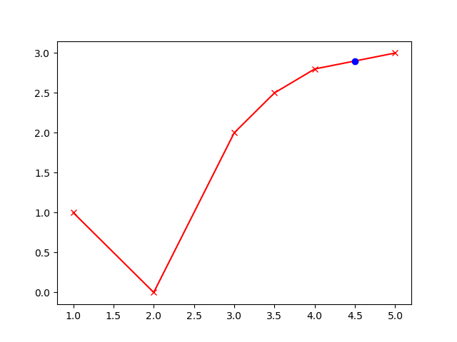
xp_val = np.array([1, 2, 3, 3.5, 4, 5])
yp_val = np.array([1, 0, 2, 2.5, 2.8, 3])
xp = [m.Param(value=xp_val[i]) for i in range(6)]
yp = [m.Param(value=yp_val[i]) for i in range(6)]
x = [m.Var(lb=xp[i],ub=xp[i+1]) for i in range(5)]
x[0].lower = -1e20
x[-1].upper = 1e20
# Variables
slk_u = [m.Var(value=1,lb=0) for i in range(4)]
slk_l = [m.Var(value=1,lb=0) for i in range(4)]
# Intermediates
slope = []
for i in range(5):
slope.append(m.Intermediate((yp[i+1]-yp[i]) / (xp[i+1]-xp[i])))
y = []
for i in range(5):
y.append(m.Intermediate((x[i]-xp[i])*slope[i]))
for i in range(4):
m.Obj(slk_u[i] + slk_l[i])
m.Equation(xz == x[0] + slk_u[0])
for i in range(3):
m.Equation(xz == x[i+1] + slk_u[i+1] - slk_l[i])
m.Equation(xz == x[4] - slk_l[3])
m.Equation(yz == yp[0] + y[0] + y[1] + y[2] + y[3] + y[4])
m.solve()
plt.plot(xp,yp,'rx-',label='PWL function')
plt.plot(xz,yz,'bo',label='Data')
plt.show()
from gekko import GEKKO
import numpy as np
m = GEKKO()
m.options.SOLVER = 1
xz = m.FV(value = 4.5)
yz = m.Var()
xp_val = np.array([1, 2, 3, 3.5, 4, 5])
yp_val = np.array([1, 0, 2, 2.5, 2.8, 3])
xp = [m.Param(value=xp_val[i]) for i in range(6)]
yp = [m.Param(value=yp_val[i]) for i in range(6)]
x = [m.Var(lb=xp[i],ub=xp[i+1]) for i in range(5)]
x[0].lower = -1e20
x[-1].upper = 1e20
# Variables
slk_u = [m.Var(value=1,lb=0) for i in range(4)]
slk_l = [m.Var(value=1,lb=0) for i in range(4)]
# Intermediates
slope = []
for i in range(5):
slope.append(m.Intermediate((yp[i+1]-yp[i]) / (xp[i+1]-xp[i])))
y = []
for i in range(5):
y.append(m.Intermediate((x[i]-xp[i])*slope[i]))
for i in range(4):
m.Obj(slk_u[i] + slk_l[i])
m.Equation(xz == x[0] + slk_u[0])
for i in range(3):
m.Equation(xz == x[i+1] + slk_u[i+1] - slk_l[i])
m.Equation(xz == x[4] - slk_l[3])
m.Equation(yz == yp[0] + y[0] + y[1] + y[2] + y[3] + y[4])
m.solve()
plt.plot(xp,yp,'rx-',label='PWL function')
plt.plot(xz,yz,'bo',label='Data')
plt.show()
Piece-wise Function with Lookup Object
! Piece-wise function with the LOOKUP object
! create the csv file
File m.csv
input, y[1], y[2]
1, 2, 4
3, 4, 6
5, -5, -7
-1, 1, 0.5
End File
! define lookup object m
Objects
m = lookup
End Objects
! connect m properties with model parameters
Connections
x = m.input
y[1] = m.y[1]
y[2] = m.y[2]
End Connections
! simple model
Model n
Parameters
x = 1
y[1]
y[2]
End Parameters
Variables
y
End Variables
Equations
y = y[1]+y[2]
End Equations
End Model