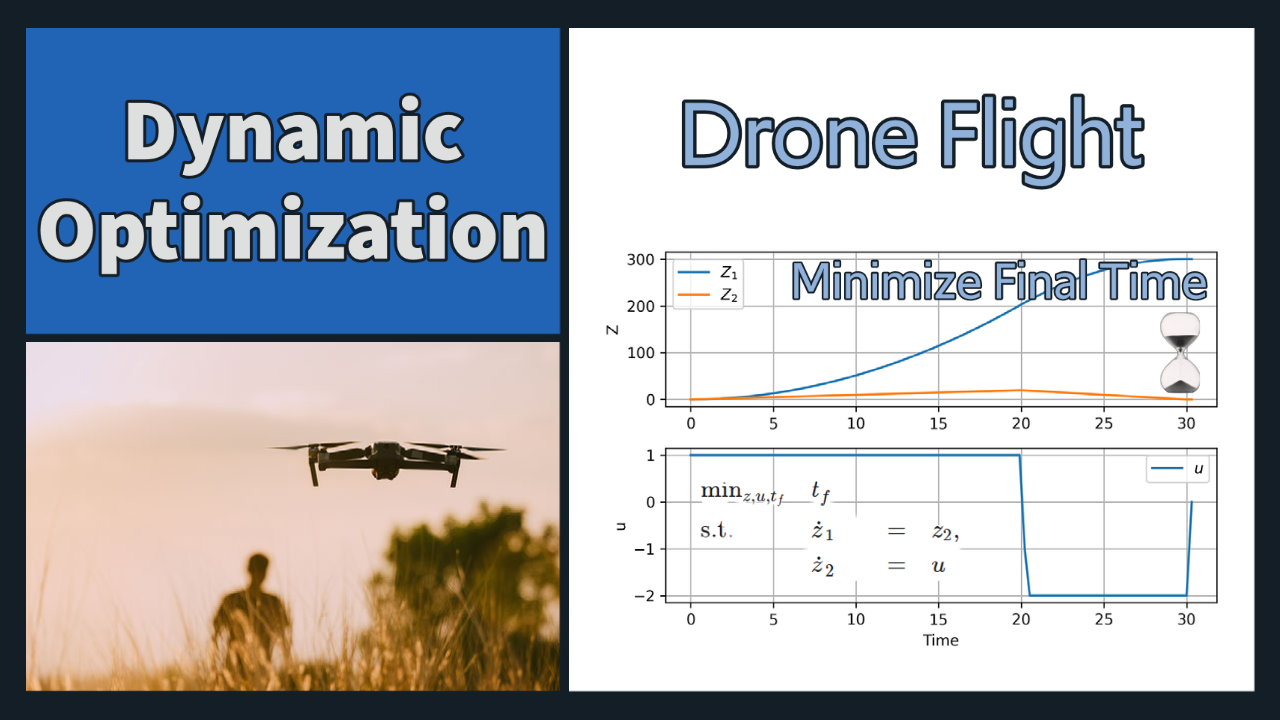
Optimal Drone Acceleration
Drone flight optimization is a critical aspect of modern UAV operations, as it can help to maximize the efficiency and effectiveness while minimizing risk and improving safety. Some objectives include reduced flight time, increased payload capacity, improved battery life, or minimized risk.
Drone flight optimization can use model predictive control (MPC) to optimize flight paths in real-time. MPC accounts for a range of factors such as wind speed and direction, altitude, and obstacles, to determine the most efficient and safest route for the drone to follow. If fast enough, MPC can adjust the drone flight path real-time to avoid obstacles or take advantage of changing weather conditions.
This simplified problem is to optimize the time for a drone to achieve a fixed distance of 300 units in minimum time to a stationary target.
$$ \begin{array}{llclr} \min_{z, u, t_f} & t_f \\ \mbox{s.t.} & \dot{z}_1 & = & z_2 \\ & \dot{z}_2 & = & u \\ & z(0) &=& (0,0)^T \\ & z(t_f) &=& (300,0)^T \\ & 0 & \leq & z_1(t) \leq 330\\ & 0 & \leq & z_2(t) \leq 33 \\ & u(t) & \in & [-2,1]\\ \end{array} $$
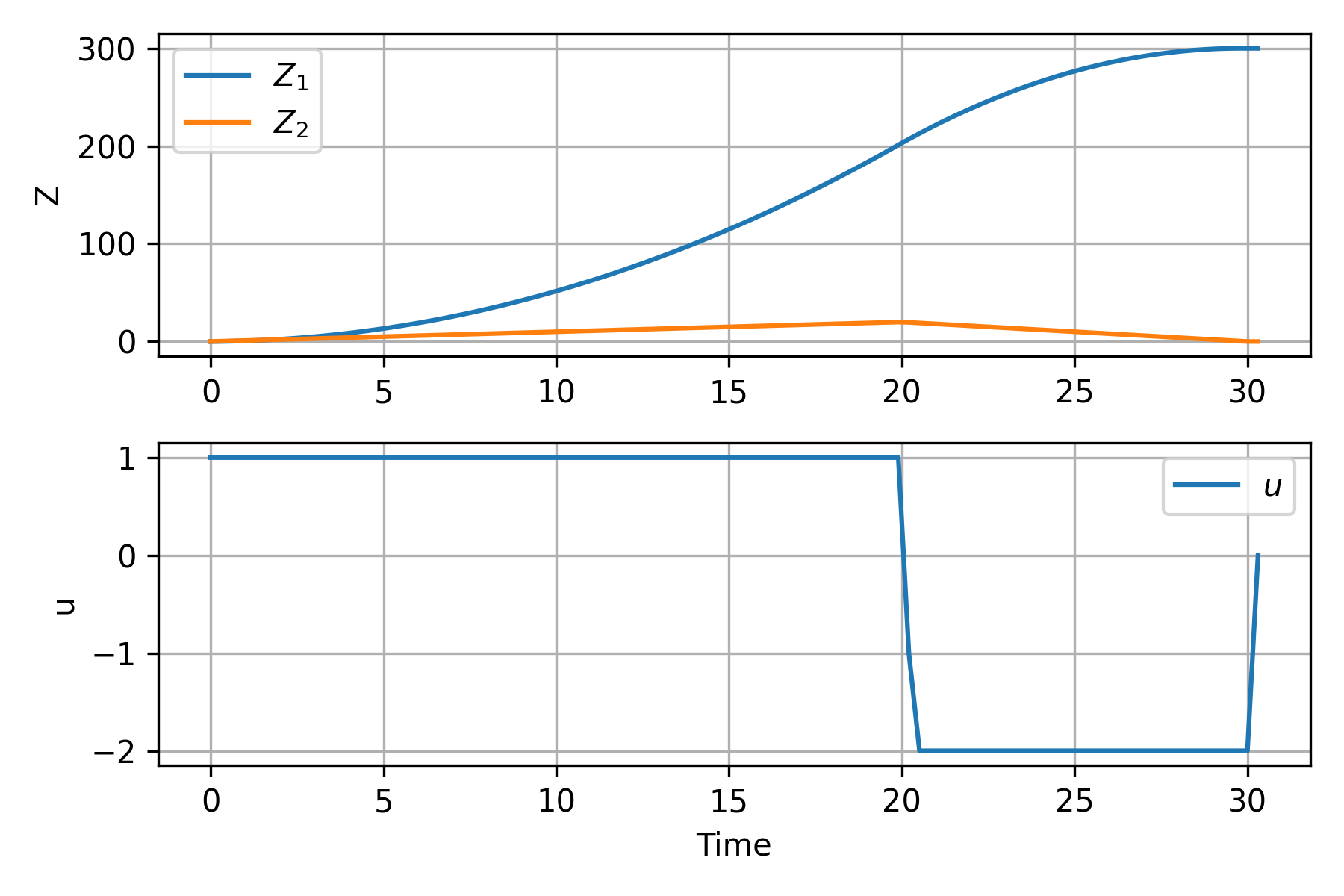
with `z = (z_1, z_2)^T`. The optimal solution is to accelerate forward until a switch point where the drone decelerates to arrive at the final target distance with zero velocity.
import matplotlib.pyplot as plt
import numpy as np
m = GEKKO(remote=False)
m.time = np.linspace(0, 1, 100)
# variables
Z1 = m.Var(value=0, ub=330, lb=0)
Z2 = m.Var(value=0, ub=33, lb=0)
m.fix_final(Z2, 0)
m.fix_final(Z1, 300)
# adjust final time
tf = m.FV(value=500, lb=0.1)
tf.STATUS = 1
# discrete decision - manipulated variable
u = m.MV(value=1, lb=-2, ub=1, integer=True)
u.STATUS = 1
m.Equation(Z1.dt() / tf == Z2)
m.Equation(Z2.dt() / tf == u)
m.Minimize(tf)
# options
m.options.IMODE = 6
m.options.SOLVER = 1
m.solve(disp=False)
# display solution
print("Total time: " + str(tf.value[0]))
tm = m.time * tf.value[0]
plt.figure(figsize=(6,4))
plt.subplot(211)
plt.plot(tm, Z1, label=r'$Z_1$')
plt.plot(tm, Z2, label=r'$Z_2$')
plt.ylabel('Z'); plt.legend(); plt.grid()
plt.subplot(212)
plt.plot(tm, u, label=r'$u$')
plt.ylabel('u'); plt.xlabel('Time')
plt.legend(); plt.grid(); plt.tight_layout()
plt.savefig('optimal_time.png',dpi=300); plt.show()
An MINLP solution is calculated with the APOPT solver with a minimized time of 30.31. Thanks to Tanner Jasperson for providing a solution.
The Gekko Optimization Suite is a machine learning and optimization package in Python for mixed-integer and differential algebraic equations.
📄 Gekko Publication and References
The GEKKO package is available in Python with pip install gekko. There are additional example problems for equation solving, optimization, regression, dynamic simulation, model predictive control, and machine learning.