Wire in Pipe for Drill Shaft Communication
Drill Shaft Communication
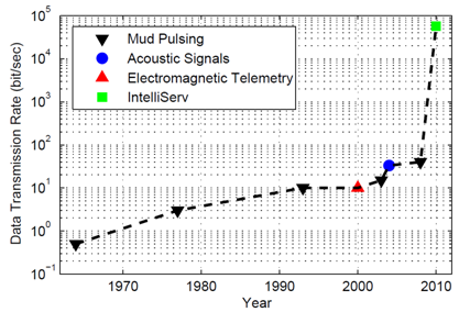
Measurement technology is advancing in the oil and gas industry. Innovations such as wireless transmitters, reduced cost of measurement technology, and increased regulations that require active monitoring have the effect of increasing the number of available measurements. Increased bandwidth does not necessarily lead to improved operations. Some describe this as Drowning in Data, Starving for Information.
This flood of information can be distilled into relevant and actionable information with Advanced Process Monitoring. The purpose of APM is to validate measurements and align imperfect mathematical models to the actual process. The objective of this approach is to determine a best estimate of the current state of the process and any potential disturbances. The opportunity is in earlier detection of disturbances, process equipment faults, and improved state estimates for optimization and control.
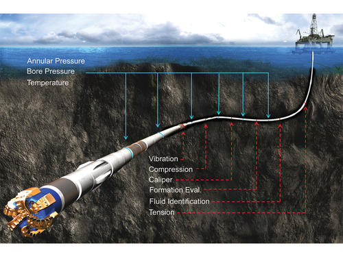
Below is a simple example of a mathematical model of inductor-connected wire-in-pipe technology provided by IntelliServ, a joint venture between Slumberger and NOV. The model describes the behavior of the communication platform in transmitting signals from the Bottom Hole Assembly (BHA) to the top-side computers.
! APMonitor Modeling Language

! Parameters include resistance (ohm), winding inductance (henrys)
Model pipe
  Parameters
    ! communication parameters
    v_in = 0      ! input voltage (Volt)
    R = 0.1       ! resistance (Ohm)
    L = 1e-5      ! inductance (Henry)
    C = 1e-8      ! capacitance (Farad)

    t[1] = 23     ! temperature in first pipe segment (°C)
    t[2:10] = t[1:9] + 10  ! temperature increases by 10°C with each segment

    n[1:10] = 100 ! number of windings on each pipe segment
                  ! can modify for different number of windings on each end
  End Parameters

  Variables
    i[1:10] = 0   ! current (Amps)
    v[1:10] = 0   ! voltage (Volt)
  End Variables

  Intermediates
    ! loss across pipe connections (dB)
    ! linear correlation (20°C = 0.5 dB, 120°C = 1.5 dB)
    dB[1:10] = (t[1:10] - 20) * (1.5-0.5)/(120-20) + 0.5

    ! inductor to inductor transfer efficiency
    eff[1:10] = 10^(-db[1:10]/20), >=0, <=1
    eff_avg[1:9] = (eff[1:9] + eff[2:10]) / 2
  End Intermediates

  Equations
    ! input voltage effect on current in 1st pipe
    L*$i[1] = -R*i[1] + v_in

    ! current dynamics in each segment
    L*$i[2:10] = -R*i[2:10] + (n[2:10]/n[1:9]) * v[1:9] * eff_avg[1:9]

    ! voltage dynamics from capacitance
    C * $v[1:10] = i[1:10] - v[1:10]/R
  End Equations

End Model
Contact support@apmonitor.com to learn more about Advanced Process Monitoring for upstream drilling and production systems.