Solve Differential Equations in Python
Main.PythonDynamicSim History
Hide minor edits - Show changes to markup
Differential equations can be solved with different methods in Python. Below are examples that show how to solve differential equations with (1) GEKKO Python, (2) Euler's method, (3) the ODEINT function from Scipy.Integrate. Additional information is provided on using APM Python for parameter estimation with dynamic models and scale-up to large-scale problems.
Differential equations can be solved with different methods in Python. Below are examples that show how to solve differential equations with (1) GEKKO Python, (2) Euler's method, (3) the ODEINT function from Scipy.Integrate. Additional information is provided on using APM Python for parameter estimation with dynamic models and scale-up to large-scale problems.
(:html:)
 <div id="disqus_thread"></div>
    <script type="text/javascript">
        /* * * CONFIGURATION VARIABLES: EDIT BEFORE PASTING INTO YOUR WEBPAGE * * */
        var disqus_shortname = 'apmonitor'; // required: replace example with your forum shortname

        /* * * DON'T EDIT BELOW THIS LINE * * */
        (function() {
            var dsq = document.createElement('script'); dsq.type = 'text/javascript'; dsq.async = true;
            dsq.src = 'https://' + disqus_shortname + '.disqus.com/embed.js';
            (document.getElementsByTagName('head')[0] || document.getElementsByTagName('body')[0]).appendChild(dsq);
        })();
    </script>
    <noscript>Please enable JavaScript to view the <a href="https://disqus.com/?ref_noscript">comments powered by Disqus.</a></noscript>
    <a href="https://disqus.com" class="dsq-brlink">comments powered by <span class="logo-disqus">Disqus</span></a>
(:htmlend:)
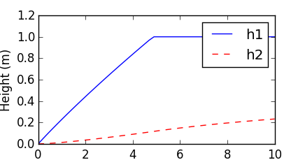
GEKKO Python solves the differential equations with tank overflow conditions. When the first tank overflows, the liquid is lost and does not enter tank 2. The model is composed of variables and equations. The differential variables (h1 and h2) are solved with a mass balance on both tanks.
See Introduction to GEKKO for more information on solving differential equations in Python. GEKKO Python solves the differential equations with tank overflow conditions. When the first tank overflows, the liquid is lost and does not enter tank 2. The model is composed of variables and equations. The differential variables (h1 and h2) are solved with a mass balance on both tanks.
See Introduction to Using ODEINT for more information on solving differential equations with SciPy.
See Introduction to ODEINT for more information on solving differential equations with SciPy.
1. GEKKO Python
1. GEKKO Python
GEKKO Python solves the differential equations with tank overflow conditions. When the first tank overflows, the liquid is lost and does not enter tank 2. The model is composed of variables and equations. The differential variables (h1 and h2) are solved with a mass balance on both tanks.
(:source lang=python:) import numpy as np import matplotlib.pyplot as plt from gekko import GEKKO
m = GEKKO()
- integration time points
m.time = np.linspace(0,10)
- constants
c1 = 0.13 c2 = 0.20 Ac = 2 # m^2
- inflow
qin1 = 0.5 # m^3/hr
- variables
h1 = m.Var(value=0,lb=0,ub=1) h2 = m.Var(value=0,lb=0,ub=1) overflow1 = m.Var(value=0,lb=0) overflow2 = m.Var(value=0,lb=0)
- outflow equations
qin2 = m.Intermediate(c1 * h1**0.5) qout1 = m.Intermediate(qin2 + overflow1) qout2 = m.Intermediate(c2 * h2**0.5 + overflow2)
- mass balance equations
m.Equation(Ac*h1.dt()==qin1-qout1) m.Equation(Ac*h2.dt()==qin2-qout2)
- minimize overflow
m.Obj(overflow1+overflow2)
- set options
m.options.IMODE = 6 # dynamic optimization
- simulate differential equations
m.solve()
- plot results
plt.figure(1) plt.plot(m.time,h1,'b-') plt.plot(m.time,h2,'r--') plt.xlabel('Time (hrs)') plt.ylabel('Height (m)') plt.legend(['height 1','height 2']) plt.show() (:sourceend:)
Differential equations can be solved with different methods in Python. Below are examples that show how to solve differential equations with (1) Euler's method, (2) the ODEINT function from Scipy.Integrate, and (3) APM Python.
Differential equations can be solved with different methods in Python. Below are examples that show how to solve differential equations with (1) GEKKO Python, (2) Euler's method, (3) the ODEINT function from Scipy.Integrate. Additional information is provided on using APM Python for parameter estimation with dynamic models and scale-up to large-scale problems.
1. Discretize with Euler's Method
1. GEKKO Python
2. Discretize with Euler's Method
(:sourceend:0
2. SciPy.Integrate ODEINT Function
(:sourceend:)
3. SciPy.Integrate ODEINT Function
3. APM Python DAE Integrator and Optimizer
APM Python DAE Integrator and Optimizer
4. ODEINT Scale-up for Large Sets of Equations
Scale-up for Large Sets of Equations
 import numpy as np
 import matplotlib.pyplot as plt

 def tank(c1,c2):
   Ac = 2 # m^2
   qin = 0.5 # m^3/hr
   dt = 0.5 # hr
   tf = 10.0 # hr

   h1 = 0
   h2 = 0
   t = 0
   ts = np.empty(21)
   h1s = np.empty(21)
   h2s = np.empty(21)
   i = 0
   while t<=10.0:
      ts[i] = t
      h1s[i] = h1
      h2s[i] = h2

      qout1 = c1 * pow(h1,0.5)
      qout2 = c2 * pow(h2,0.5)
      h1 = (qin-qout1)*dt/Ac + h1
      if h1>1:
         h1 = 1
      h2 = (qout1-qout2)*dt/Ac + h2
      i = i + 1
      t = t + dt

   # plot data
   plt.figure(1)
   plt.plot(ts,h1s)
   plt.plot(ts,h2s)
   plt.xlabel("Time (hrs)")
   plt.ylabel("Height (m)")
   plt.show()

 # call function
 tank(0.13,0.20)
(:source lang=python:) import numpy as np import matplotlib.pyplot as plt
def tank(c1,c2):
  Ac = 2 # m^2
  qin = 0.5 # m^3/hr
  dt = 0.5 # hr
  tf = 10.0 # hr

  h1 = 0
  h2 = 0
  t = 0
  ts = np.empty(21)
  h1s = np.empty(21)
  h2s = np.empty(21)
  i = 0
  while t<=10.0:
     ts[i] = t
     h1s[i] = h1
     h2s[i] = h2

     qout1 = c1 * pow(h1,0.5)
     qout2 = c2 * pow(h2,0.5)
     h1 = (qin-qout1)*dt/Ac + h1
     if h1>1:
        h1 = 1
     h2 = (qout1-qout2)*dt/Ac + h2
     i = i + 1
     t = t + dt

  # plot data
  plt.figure(1)
  plt.plot(ts,h1s)
  plt.plot(ts,h2s)
  plt.xlabel("Time (hrs)")
  plt.ylabel("Height (m)")
  plt.show()
- call function
tank(0.13,0.20) (:sourceend:0
See Introduction to Using ODEINT for more information on solving differential equations with SciPy.
 import numpy as np
 import matplotlib.pyplot as plt
 from scipy.integrate import odeint

 def tank(h,t):
    # constants
    c1 = 0.13
    c2 = 0.20
    Ac = 2      # m^2
    # inflow
    qin = 0.5   # m^3/hr
    # outflow
    qout1 = c1 * h[0]**0.5
    qout2 = c2 * h[1]**0.5
    # differential equations
    dhdt1 = (qin   - qout1) / Ac
    dhdt2 = (qout1 - qout2) / Ac
    # overflow conditions
    if h[0]>=1 and dhdt1>=0:
        dhdt1 = 0
    if h[1]>=1 and dhdt2>=0:
        dhdt2 = 0
    dhdt = [dhdt1,dhdt2]
    return dhdt

 # integrate the equations
 t = np.linspace(0,10) # times to report solution
 h0 = [0,0]            # initial conditions for height
 y = odeint(tank,h0,t) # integrate

 # plot results
 plt.figure(1)
 plt.plot(t,y[:,0],'b-')
 plt.plot(t,y[:,1],'r--')
 plt.xlabel('Time (hrs)')
 plt.ylabel('Height (m)')
 plt.legend(['h1','h2'])
 plt.show()
(:source lang=python:) import numpy as np import matplotlib.pyplot as plt from scipy.integrate import odeint
def tank(h,t):
   # constants
   c1 = 0.13
   c2 = 0.20
   Ac = 2      # m^2
   # inflow
   qin = 0.5   # m^3/hr
   # outflow
   qout1 = c1 * h[0]**0.5
   qout2 = c2 * h[1]**0.5
   # differential equations
   dhdt1 = (qin   - qout1) / Ac
   dhdt2 = (qout1 - qout2) / Ac
   # overflow conditions
   if h[0]>=1 and dhdt1>=0:
       dhdt1 = 0
   if h[1]>=1 and dhdt2>=0:
       dhdt2 = 0
   dhdt = [dhdt1,dhdt2]
   return dhdt
- integrate the equations
t = np.linspace(0,10) # times to report solution h0 = [0,0] # initial conditions for height y = odeint(tank,h0,t) # integrate
- plot results
plt.figure(1) plt.plot(t,y[:,0],'b-') plt.plot(t,y[:,1],'r--') plt.xlabel('Time (hrs)') plt.ylabel('Height (m)') plt.legend(['h1','h2']) plt.show() (:sourceend:)
(:htmlend:)
4. ODEINT Scale-up for Large Sets of Equations
(:html:) <iframe width="560" height="315" src="https://www.youtube.com/embed/8kx6vC9gTLo" frameborder="0" allowfullscreen></iframe>
This 5 minute tutorial gives step-by-step instructions on how to simulate dynamic systems. Dynamic systems may have differential and algebraic equations (DAEs) or just differential equations (ODEs) that cause a time evolution of the response. The tutorial covers the same problem in both MATLAB and Python.
(:html:) <iframe width="560" height="315" src="//www.youtube.com/embed/-IDTagajoyA?rel=0" frameborder="0" allowfullscreen></iframe> (:htmlend:)
The Python package Scipy offers several solvers to numerically simulate the solution of sets of differential equations. Below is an example of solving a first-order decay with the APM solver in Python. The objective is to fit the differential equation solution to data by adjusting unknown parameters until the model and measured values match.
This tutorial gives step-by-step instructions on how to simulate dynamic systems. Dynamic systems may have differential and algebraic equations (DAEs) or just differential equations (ODEs) that cause a time evolution of the response. Below is an example of solving a first-order decay with the APM solver in Python. The objective is to fit the differential equation solution to data by adjusting unknown parameters until the model and measured values match.
(:html:) <iframe width="560" height="315" src="https://www.youtube.com/embed/U7uyj9BaNKg" frameborder="0" allowfullscreen></iframe> (:htmlend:)
 import numpy as np
 import matplotlib.pyplot as plt
 from scipy.integrate import odeint

 def tank(h,t):
    # constants
    c1 = 0.13
    c2 = 0.20
    Ac = 2      # m^2
    # inflow
    qin = 0.5   # m^3/hr
    # outflow
    qout1 = c1 * h[0]**0.5
    qout2 = c2 * h[1]**0.5
    # differential equations
    dhdt1 = (qin   - qout1) / Ac
    dhdt2 = (qout1 - qout2) / Ac
    # overflow conditions
    if h[0]>=1 and dhdt1>=0:
        dhdt1 = 0
    if h[1]>=1 and dhdt2>=0:
        dhdt2 = 0
    dhdt = [dhdt1,dhdt2]
    return dhdt

 # integrate the equations
 t = np.linspace(0,10) # times to report solution
 h0 = [0,0]            # initial conditions for height
 y = odeint(tank,h0,t) # integrate

 # plot results
 plt.figure(1)
 plt.plot(t,y[:,0],'b-')
 plt.plot(t,y[:,1],'r--')
 plt.xlabel('Time (hrs)')
 plt.ylabel('Height (m)')
 plt.legend(['h1','h2'])
 plt.show()
Differential equations can be solved with different methods in Python. Below are examples that show how to solve differential equations with (1) Euler's method, (2) the ODEINT function from Scipy.Integrate, and (3) APM Python.
1. Discretize with Euler's Method
DAE Integrator and Optimizer
2. SciPy.Integrate ODEINT Function
3. APM Python DAE Integrator and Optimizer
Source Code
 import numpy as np
 import matplotlib.pyplot as plt

 def tank(c1,c2):
   Ac = 2 # m^2
   qin = 0.5 # m^3/hr
   dt = 0.5 # hr
   tf = 10.0 # hr

   h1 = 0
   h2 = 0
   t = 0
   ts = np.empty(21)
   h1s = np.empty(21)
   h2s = np.empty(21)
   i = 0
   while t<=10.0:
      ts[i] = t
      h1s[i] = h1
      h2s[i] = h2

      qout1 = c1 * pow(h1,0.5)
      qout2 = c2 * pow(h2,0.5)
      h1 = (qin-qout1)*dt/Ac + h1
      if h1>1:
         h1 = 1
      h2 = (qout1-qout2)*dt/Ac + h2
      i = i + 1
      t = t + dt

   # plot data
   plt.figure(1)
   plt.plot(ts,h1s)
   plt.plot(ts,h2s)
   plt.xlabel("Time (hrs)")
   plt.ylabel("Height (m)")
   plt.show()

 # call function
 tank(0.13,0.20)
Euler's method is used to solve a set of two differential equations in Excel and Python.
(:html:) <iframe width="560" height="315" src="https://www.youtube.com/embed/ygoohjN_Lww" frameborder="0" allowfullscreen></iframe> (:htmlend:)
DAE Integrator and Optimizer
This same example problem is also demonstrated with Spreadsheet Programming and in the Matlab programming language.
Additional Material
This same example problem is also demonstrated with Spreadsheet Programming and in the Matlab programming language. Another example problem demonstrates how to calculate the concentration of CO gas buildup in a room.
- Case Study on CO Buildup in a Room
<iframe width="560" height="315" src="//www.youtube.com/embed/YvjG2LRNtKU" frameborder="0" allowfullscreen></iframe>
<iframe width="560" height="315" src="//www.youtube.com/embed/-IDTagajoyA?rel=0" frameborder="0" allowfullscreen></iframe>
<iframe width="560" height="315" src="//www.youtube.com/embed/YvjG2LRNtKU" frameborder="0" allowfullscreen></iframe>
(:title Solve Differential Equations in Python:) (:keywords introduction, Python, programming language, differential equations, nonlinear, university course:) (:description Solve Differential Equations in Python - Problem-Solving Techniques for Chemical Engineers at Brigham Young University:)
This 5 minute tutorial gives step-by-step instructions on how to simulate dynamic systems. Dynamic systems may have differential and algebraic equations (DAEs) or just differential equations (ODEs) that cause a time evolution of the response. The tutorial covers the same problem in both MATLAB and Python.
(:html:) <iframe width="560" height="315" src="//www.youtube.com/embed/YvjG2LRNtKU" frameborder="0" allowfullscreen></iframe> (:htmlend:)
The Python package Scipy offers several solvers to numerically simulate the solution of sets of differential equations. Below is an example of solving a first-order decay with the APM solver in Python. The objective is to fit the differential equation solution to data by adjusting unknown parameters until the model and measured values match.
(:html:) (:htmlend:)
This same example problem is also demonstrated with Spreadsheet Programming and in the Matlab programming language.
(:html:)
 <div id="disqus_thread"></div>
    <script type="text/javascript">
        /* * * CONFIGURATION VARIABLES: EDIT BEFORE PASTING INTO YOUR WEBPAGE * * */
        var disqus_shortname = 'apmonitor'; // required: replace example with your forum shortname

        /* * * DON'T EDIT BELOW THIS LINE * * */
        (function() {
            var dsq = document.createElement('script'); dsq.type = 'text/javascript'; dsq.async = true;
            dsq.src = 'https://' + disqus_shortname + '.disqus.com/embed.js';
            (document.getElementsByTagName('head')[0] || document.getElementsByTagName('body')[0]).appendChild(dsq);
        })();
    </script>
    <noscript>Please enable JavaScript to view the <a href="https://disqus.com/?ref_noscript">comments powered by Disqus.</a></noscript>
    <a href="https://disqus.com" class="dsq-brlink">comments powered by <span class="logo-disqus">Disqus</span></a>
(:htmlend:)
