Learn Programming

1. data

1. regression

a = m.FV(value=0); a.STATUS=1 b = m.FV(value=0); b.STATUS=1 c = m.FV(value=0,lb=-100,ub=100); c.STATUS=1

1. load data

1. define model

m.options.IMODE = 2

m = GEKKO() # remote=False for local mode

m.Minimize(((ypred-ymeas)/ymeas)**2)

m.solve()

There is additional information on regression in the Data Science online course.

While this exercise demonstrates only one independent parameter and one dependent variable, any number of independent or dependent terms can be included. See Energy Price regression with three independent variables as an example.

import numpy as np x = np.array([0,1,2,3,4,5]) y = np.array([0,0.8,0.9,0.1,-0.8,-1])

p1 = np.polyfit(x,y,1) p2 = np.polyfit(x,y,2) p3 = np.polyfit(x,y,3)

import matplotlib.pyplot as plt plt.plot(x,y,'o') xp = np.linspace(-2,6,100) plt.plot(xp,np.polyval(p1,xp),'r-') plt.plot(xp,np.polyval(p2,xp),'b--') plt.plot(xp,np.polyval(p3,xp),'m:')

SSresid = np.sum(yresid**2) SStotal = len(y) * np.var(y)

from scipy.stats import linregress

print(r_value**2)

plt.show()

(:toggle hide regression button show="Linear and Polynomial Regression Source Code":) (:div id=regression:) (:source lang=python:) from numpy import * x = array([0,1,2,3,4,5]) y = array([0,0.8,0.9,0.1,-0.8,-1]) print(x) print(y)

from scipy.interpolate import * p1 = polyfit(x,y,1) p2 = polyfit(x,y,2) p3 = polyfit(x,y,3) print(p1) print(p2) print(p3)

from matplotlib.pyplot import * plot(x,y,'o') xp = linspace(-2,6,100) plot(xp,polyval(p1,xp),'r-') plot(xp,polyval(p2,xp),'b--') plot(xp,polyval(p3,xp),'m:') yfit = p1[0] * x + p1[1] yresid= y - yfit SSresid = sum(pow(yresid,2)) SStotal = len(y) * var(y) rsq = 1 - SSresid/SStotal print(yfit) print(y) print(rsq)

from scipy.stats import * slope,intercept,r_value,p_value,std_err = linregress(x,y) print(pow(r_value,2)) print(p_value) show() (:sourceend:) (:divend:)

(:html:) <iframe width="560" height="315" src="https://www.youtube.com/embed/3ZVRstDL9A4" frameborder="0" allow="autoplay; encrypted-media" allowfullscreen></iframe> (:htmlend:)

Regression with Python (GEKKO or Scipy)

Python Data Regression

Correlations from data are obtained by adjusting parameters of a model to best fit the measured outcomes. The analysis may include statistics, data visualization, or other calculations to synthesize the information into relevant and actionable information. This tutorial demonstrates how to create a linear, polynomial, or nonlinear functions that best approximate the data and analyze the result. Script files of the Python source code with sample data are available below.

    a,b,c = x

    return np.sum(((calc_y(x)-ym)/ym)**2)

(:sourceend:)

Linear and Polynomial Regression

Regression with GEKKO

(:toggle hide gekko button show="Python GEKKO Solution":) (:div id=gekko:)

from gekko import GEKKO

1. define GEKKO model

m = GEKKO()

1. parameters and variables

a = m.FV(value=0) b = m.FV(value=0) c = m.FV(value=0,lb=-100,ub=100) x = m.Param(value=xm) ymeas = m.Param(value=ym) ypred = m.Var()

1. parameter and variable options

a.STATUS = 1 # available to optimizer b.STATUS = 1 # to minimize objective c.STATUS = 1

1. equation

m.Equation(ypred == a + b/x + c*m.log(x))

1. objective

m.Obj(((ypred-ymeas)/ymeas)**2)

1. application options

m.options.IMODE = 2 # regression mode

1. solve

m.solve() # remote=False for local solve

print('Final SSE Objective: ' + str(m.options.objfcnval))

print('a = ' + str(a.value[0])) print('b = ' + str(b.value[0])) print('c = ' + str(c.value[0]))

plt.plot(x,ymeas,'ro') plt.plot(x,ypred,'bx');

Regression with Python SciPy Optimize

(:toggle hide python_minimize button show="Python SciPy Solution":) (:div id=python_minimize:) (:source lang=python:) import numpy as np from scipy.optimize import minimize

1. load data

xm = np.array([18.3447,79.86538,85.09788,10.5211,44.4556, 69.567,8.960,86.197,66.857,16.875, 52.2697,93.917,24.35,5.118,25.126, 34.037,61.4445,42.704,39.531,29.988])

ym = np.array([5.072,7.1588,7.263,4.255,6.282, 6.9118,4.044,7.2595,6.898,4.8744, 6.5179,7.3434,5.4316,3.38,5.464, 5.90,6.80,6.193,6.070,5.737])

1. calculate y

def calc_y(x):

    a = x[0]
    b = x[1]
    c = x[2]
    y = a + b/xm + c*np.log(xm)
    return y

1. define objective

def objective(x):

    # calculate y
    y = calc_y(x)
    # calculate objective
    obj = 0.0
    for i in range(len(ym)):
        obj = obj + ((y[i]-ym[i])/ym[i])**2    
    # return result
    return obj

1. initial guesses

x0 = np.zeros(3) x0[0] = 0.0 # a x0[1] = 0.0 # b x0[2] = 0.0 # c

1. show initial objective

print('Initial SSE Objective: ' + str(objective(x0)))

1. optimize
2. bounds on variables

bnds100 = (-100.0, 100.0) no_bnds = (-1.0e10, 1.0e10) bnds = (no_bnds, no_bnds, bnds100) solution = minimize(objective,x0,method='SLSQP',bounds=bnds) x = solution.x y = calc_y(x)

1. show final objective

print('Final SSE Objective: ' + str(objective(x)))

1. print solution

print('Solution') print('a = ' + str(x[0])) print('b = ' + str(x[1])) print('c = ' + str(x[2]))

1. plot solution

import matplotlib.pyplot as plt plt.figure(1) plt.plot(xm,ym,'ro') plt.plot(xm,y,'bx'); plt.xlabel('x') plt.ylabel('y') plt.legend(['Measured','Predicted'],loc='best') plt.savefig('results.png') plt.show() (:sourceend:) (:divend:)

Regression with APM Python

• APM Python Nonlinear Regression Example Source Code

(:html:) <iframe width="560" height="315" src="https://www.youtube.com/embed/EShuLfSxpsI" frameborder="0" allowfullscreen></iframe> (:htmlend:)

Excel and MATLAB

This regression tutorial can also be completed with Excel and Matlab. A multivariate nonlinear regression case with multiple factors is available with example data for energy prices in Python. Click on the appropriate link for additional information.

(:toggle hide python_minimize button show="Python SciPy Solution":) (:div id=python_minimize:)

(:divend:)

xm = np.array([18.3447,79.86538,85.09788,10.5211,44.4556, 69.567,8.960,86.197,66.857,16.875, 52.2697,93.917,24.35,5.118,25.126, 34.037,61.4445,42.704,39.531,29.988])

ym = np.array([5.072,7.1588,7.263,4.255,6.282, 6.9118,4.044,7.2595,6.898,4.8744, 6.5179,7.3434,5.4316,3.38,5.464, 5.90,6.80,6.193,6.070,5.737])

Nonlinear Regression with APM Python

• APM Python Nonlinear Regression Example Source Code

Nonlinear Regression with Python SciPy Optimize

(:source lang=python:) import numpy as np from scipy.optimize import minimize

1. load data

xm = np.array([18.34470085,79.86537666,85.09787509,10.52110327,44.45558653, 69.56726251,8.959848679,86.196964,66.85655694,16.87490807, 52.26970696,93.91681982,24.34668842,5.117815482,25.12622222, 34.03722832,61.44454908,42.703577,39.53089298,29.98844942])

ym = np.array([5.072227705,7.15881537,7.262764628,4.254581322,6.281866658, 6.911787335,4.043809747,7.259528698,6.898089228,4.874417979, 6.517943774,7.343419502,5.431648634,3.384634319,5.464227719, 5.90043173,6.803895621,6.193263135,6.070397707,5.736792474])

1. calculate y

def calc_y(x):

    a = x[0]
    b = x[1]
    c = x[2]
    y = a + b/xm + c*np.log(xm)
    return y

1. define objective

def objective(x):

    # calculate y
    y = calc_y(x)
    # calculate objective
    obj = 0.0
    for i in range(len(ym)):
        obj = obj + ((y[i]-ym[i])/ym[i])**2    
    # return result
    return obj

1. initial guesses

x0 = np.zeros(3) x0[0] = 0.0 # a x0[1] = 0.0 # b x0[2] = 0.0 # c

1. show initial objective

print('Initial SSE Objective: ' + str(objective(x0)))

1. optimize
2. bounds on variables

bnds100 = (-100.0, 100.0) no_bnds = (-1.0e10, 1.0e10) bnds = (no_bnds, no_bnds, bnds100) solution = minimize(objective,x0,method='SLSQP',bounds=bnds) x = solution.x y = calc_y(x)

1. show final objective

print('Final SSE Objective: ' + str(objective(x)))

1. print solution

print('Solution') print('a = ' + str(x[0])) print('b = ' + str(x[1])) print('c = ' + str(x[2]))

1. plot solution

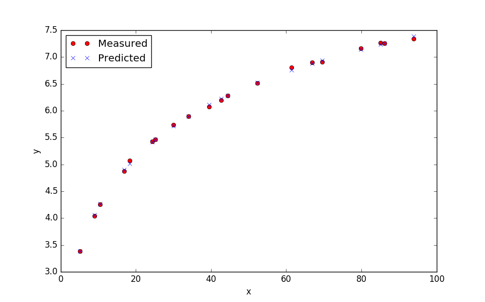
import matplotlib.pyplot as plt plt.figure(1) plt.plot(xm,ym,'ro') plt.plot(xm,y,'bx'); plt.xlabel('x') plt.ylabel('y') plt.legend(['Measured','Predicted'],loc='best') plt.savefig('results.png') plt.show() (:sourceend:)

<iframe width="560" height="315" src="https://www.youtube.com/embed/EShuLfSxpsI" frameborder="0" allowfullscreen></iframe>

Linear and Polynomial Regression

(:html:) <iframe width="560" height="315" src="https://www.youtube.com/embed/ro5ftxuD6is" frameborder="0" allowfullscreen></iframe> (:htmlend:)

Nonlinear Regression

• Python Nonlinear Regression Example Source Code

This regression tutorial can also be completed with Excel and Matlab. Click on the appropriate link for additional information.

(:title Data Regression with Python:) (:keywords data regression, Python, numpy, spreadsheet, nonlinear, polynomial, linear regression, university course:) (:description Data Regression with Python - Problem-Solving Techniques for Chemical Engineers at Brigham Young University:)

Python Data Regression

A frequent activity for scientists and engineers is to develop correlations from data. By importing the data into Python, data analysis such as statistics, trending, or calculations can be made to synthesize the information into relevant and actionable information. This tutorial demonstrates how to create a linear or polynomial functions that best approximate the data trend, plot the results, and perform a basic statistical analysis. A script file of the Python source code with sample data is below.

• Python Data Regression Example Source Code

(:html:) <iframe width="560" height="315" src="https://www.youtube.com/embed/ro5ftxuD6is" frameborder="0" allowfullscreen></iframe> (:htmlend:)

This tutorial can also be completed with Excel and Matlab. Click on the appropriate link for additional information.

(:html:)

 <div id="disqus_thread"></div>
    <script type="text/javascript">
        /* * * CONFIGURATION VARIABLES: EDIT BEFORE PASTING INTO YOUR WEBPAGE * * */
        var disqus_shortname = 'apmonitor'; // required: replace example with your forum shortname

        /* * * DON'T EDIT BELOW THIS LINE * * */
        (function() {
            var dsq = document.createElement('script'); dsq.type = 'text/javascript'; dsq.async = true;
            dsq.src = 'https://' + disqus_shortname + '.disqus.com/embed.js';
            (document.getElementsByTagName('head')[0] || document.getElementsByTagName('body')[0]).appendChild(dsq);
        })();
    </script>
    <noscript>Please enable JavaScript to view the <a href="https://disqus.com/?ref_noscript">comments powered by Disqus.</a></noscript>
    <a href="https://disqus.com" class="dsq-brlink">comments powered by <span class="logo-disqus">Disqus</span></a>

(:htmlend:)