Simulation
Main.Simulation History
Hide minor edits - Show changes to markup
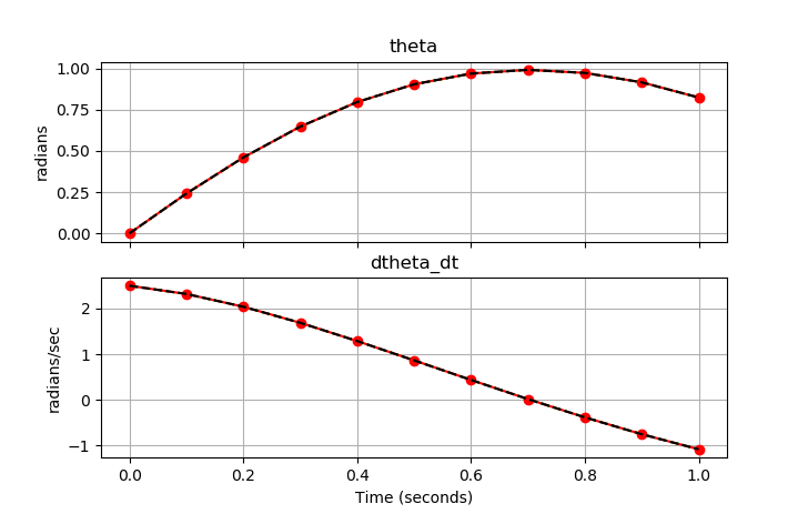
Three simulations show simultaneous simulation (IMODE=4), sequential simulation (IMODE=7), and simultaneous simulation in a Python loop (IMODE=4).
Dynamic simulation is the easiest dynamic mode to configure and run. The requirement for a square problem facilitates model convergence as the solver has only to achieve feasibility with the equality constraints.
Dynamic simulation is the easiest dynamic mode to configure and run. The requirement for a square problem facilitates model convergence as the solver has only to achieve feasibility with the equality constraints.
Example Code (Python GEKKO) with IMODE 4 and 7
(:source lang=python:) from gekko import GEKKO import numpy as np import matplotlib.pyplot as plt
- Number of timesteps
nt = 11 tm = np.linspace(0, 1, nt)
- Initialize GEKKO
p1 = GEKKO() p2 = GEKKO() p3 = GEKKO()
- define model
for p in [p1,p2,p3]:
    if p==p3:
        p.time = [tm[0],tm[1]]
    else:
        p.time = tm

    # Model parameters
    p.g = p.Const(value=9.81, name='g')
    p.l = p.Const(value=2., name='length')
    p.m = p.Const(value=1.0, name='mass')
    p.f = p.Const(value=0.5, name='friction coefficient')

    # State Variables
    p.theta = p.Var(value=0, name='angle')
    p.dtheta_dt = p.Var(value=2.5, name='angular velocity')

    # Equations
    p.Equation(p.theta.dt() == p.dtheta_dt)
    p.Equation(p.dtheta_dt.dt() ==                -p.g/p.l*p.sin(p.theta) - p.f/p.m*p.dtheta_dt)
    p.options.NODES=5
- Solve simultaneously
p1.options.IMODE=4 p1.solve(disp=False)
p2.options.IMODE=7 p2.solve(disp=False)
p3.options.IMODE=4 th = np.ones_like(tm) dth = np.ones_like(tm) th[0] = 0 dth[0] = 2.5 import time for i in range(1,nt):
    p3.solve(disp=False)

    # record values for plotting
    th[i] = p3.theta.value[1]
    dth[i] = p3.dtheta_dt.value[1]
- Plot results
fig, axes = plt.subplots(2, 1, sharex=True, figsize=(8,7))
axes[0].plot(tm, p1.theta.value, 'o-',color='red') axes[0].plot(tm, p2.theta.value, ':',color='green') axes[0].plot(tm, th, ,color='black') axes[0].set_title("theta") axes[0].set_ylabel('radians') axes[0].grid()
axes[1].plot(tm, p1.dtheta_dt.value, 'o-',color='red') axes[1].plot(tm, p2.dtheta_dt.value, ':',color='green') axes[1].plot(tm, dth, ,color='black') axes[1].set_title("dtheta_dt") axes[1].set_ylabel('radians/sec') axes[1].grid() axes[1].set_xlabel('Time (seconds)')
plt.show() (:sourceend:)
 nlc.imode = 4 (simultaneous dynamic simulation)
 nlc.imode = 7 (sequential dynamic simulation)
 apm.imode = 4 (simultaneous dynamic simulation)
 apm.imode = 7 (sequential dynamic simulation)
apm_option(server,app,'nlc.imode',7);
apm_option(server,app,'apm.imode',7);
apm_option(server,app,'nlc.imode',4)
apm_option(server,app,'apm.imode',4)
 NLC.imode = 4
 or
 NLC.imode = 7
 nlc.imode = 4 (simultaneous dynamic simulation)
 nlc.imode = 7 (sequential dynamic simulation)

 % MATLAB example
 apm_option(server,app,'nlc.imode',7);

 # Python example
 apm_option(server,app,'nlc.imode',4)
The DBS file parameter imode is used to control the simulation mode. This option is set to 4 for dynamic simulation.
NLC.imode = 4
The DBS file parameter imode is used to control the simulation mode. This option is set to 4 (simultaneous simulation) or 7 (sequential simulation) for dynamic simulation.
 NLC.imode = 4
 or
 NLC.imode = 7
NLC.imode = 4
NLC.imode = 4
Like steady-state simulation, dynamic simulation requires a square problem with no degrees of freedom (neqn=nvar). Dynamic simulation has many useful purposes including
- Investigate step response characteristics of a nonlinear model
- Simulate process changes for design, trouble-shooting, or planning
- Perform what-if scenarios
- Simulate a virtual process
Dynamic simulation is the easiest dynamic mode to configure and run. The requirement for a square problem facilitates model convergence as the solver has only to achieve feasibility with the equality constraints.
Dynamic Simulation
The DBS file parameter imode is used to control the simulation mode. This option is set to 4 for dynamic simulation.
NLC.imode = 4