APMonitor

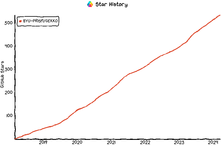
Gekko source code is available on GitHub. It is downloaded 330,000 times per month according to PyPi stats.

(:html:) <a class="github-button" href="https://github.com/BYU-PRISM/GEKKO" data-color-scheme="no-preference: light; light: light; dark: dark;" data-icon="octicon-star" data-size="large" data-show-count="true" aria-label="Star BYU-PRISM/GEKKO on GitHub">Star</a>

<script async defer src="https://buttons.github.io/buttons.js"></script> (:htmlend:)

(:html:) <a href='https://colab.research.google.com/github/BYU-PRISM/GEKKO/blob/master/examples/gekko_18examples.ipynb'> <button class="button"><span>Try Gekko Online</span></button> </a> (:htmlend:)

(:htmlend:)

(:html:) <style> .button {

  border-radius: 4px;
  background-color: #0066ff;
  border: none;
  color: #FFFFFF;
  text-align: center;
  font-size: 24px;
  padding: 20px;
  width: 100%;
  transition: all 0.5s;
  cursor: pointer;
  margin: 5px;

}

.button span {

  cursor: pointer;
  display: inline-block;
  position: relative;
  transition: 0.5s;

}

.button span:after {

  content: '\00bb';
  position: absolute;
  opacity: 0;
  top: 0;
  right: -20px;
  transition: 0.5s;

}

.button:hover span {

  padding-right: 25px;

}

.button:hover span:after {

  opacity: 1;
  right: 0;

}

.button2 {

  border-radius: 4px;
  background-color: #0066ff;
  border: none;
  color: #FFFFFF;
  text-align: center;
  font-size: 24px;
  padding: 20px;
  width: 100%;
  transition: all 0.5s;
  cursor: pointer;
  margin: 5px;

}

.button2 span {

  cursor: pointer;
  display: inline-block;
  position: relative;
  transition: 0.5s;

}

.button2 span:after {

  content: '\00bb';
  position: absolute;
  opacity: 0;
  top: 0;
  right: -20px;
  transition: 0.5s;

}

.button2:hover span {

  padding-right: 25px;

}

.button2:hover span:after {

  opacity: 1;
  right: 0;

} </style>

nt=51 # number of time steps m.time = np.linspace(0,10,nt)

1. input steps

u_meas = np.zeros(nt)

1. simulated measurements

y_meas = (np.random.rand(nt)-0.5)*0.2

m.solve(disp=True)

The latest GEKKO source is available on GitHub. Download statistics are available from the PyPI Stats Website. Functionality is tested with Python 2.7 and Python 3+ for all operating systems (Windows, MacOS, Linux) and architectures (such as ARM processors) that support Python.

Hybrid Machine Learning: Cosine Activation

Gekko Brain Module Simplifies Code

Hybrid Machine Learning: Cosine Activation

Gekko Brain Module Simplifies Code

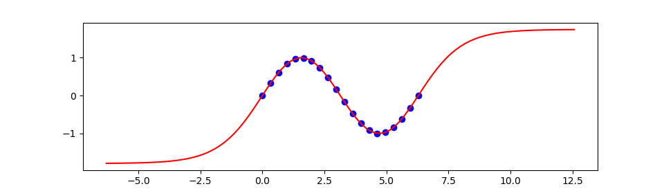
(:source lang=python:) from gekko import brain import numpy as np import matplotlib.pyplot as plt

1. generate training data

x = np.linspace(0.0,2*np.pi,20) y = np.sin(x)

x = np.array(x) y = np.array(y)

b = brain.Brain() b.input_layer(1) b.layer(linear=2) b.layer(tanh=3) b.layer(linear=2) b.output_layer(1)

b.learn(x,y) # train xp = np.linspace(-2*np.pi,4*np.pi,100) yp = b.think(xp) # validate

plt.figure() plt.plot(x,y,'bo') plt.plot(xp,yp[0],'r-') plt.show() (:sourceend:)

Hybrid Machine Learning: Cosine Activation Function

(:title GEKKO Python Tutorials:)

from gekko import GEKKO

 pip install gekko

m.solve(disp=False)

m.solve()

m.solve(disp=True)

• (:html:)<a href='https://en.wikipedia.org/wiki/Gekko_(optimization_software)'>GEKKO Wikipedia Article</a>(:htmlend:)

 python -m pip install gekko

m.open_folder()

    n2 = 2   # hidden layer 2 (nonlinear)

GEKKO Python is designed for large-scale optimization and accesses solvers of constrained, unconstrained, continuous, and discrete problems. Problems in linear programming, quadratic programming, integer programming, nonlinear optimization, systems of dynamic nonlinear equations, and multi-objective optimization can be solved. The platform can find optimal solutions, perform tradeoff analyses, balance multiple design alternatives, and incorporate optimization methods into external modeling and analysis software. It is free for academic and commercial use under the MIT license.

x1.lower = 1 x2.lower = 1 x3.lower = 1 x4.lower = 1

x1.upper = 5 x2.upper = 5 x3.upper = 5 x4.upper = 5

There are many other applications and instructional material posted to this freely available course web-site. The online course is generally offered starting each year in January. There are two course projects that include the advanced temperature control lab (1st project) and a project that is a group choice (2nd project). Below is an example student presentation at the end of the course. It is representative of the modeling, estimation, and control methods that are taught in the dynamic optimization course.

The Dynamic Optimization Course is graduate level course taught in three modules to introduce concepts in:

• mathematical modeling (3 weeks)
• machine learning, estimation (3 weeks)
• control, optimization (3 weeks)

There are many other applications and instructional material posted to this freely available course web-site. The online course is generally offered starting each year in January. There are two course projects that include the temperature control lab (1st project) and a project that is a group choice (2nd project)). Below is an example student presentation at the end of the course. It is representative of the modeling, estimation, and control methods that are taught in the course.

There are 18 example problems with GEKKO that are provided below. These examples demonstrate the equation solving, regression, differential equation simulation, nonlinear programming, machine learning, model predictive control, moving horizon estimation, debugging, and other applications. While these applications are designed to be tutorial in nature and very simple, GEKKO references are further application examples of complex and multi-disciplinary systems.

GEKKO Information

The latest GEKKO source is available on Github. Functionality is tested with Python 2.7 and Python 3+ for all operating systems (Windows, MacOS, Linux) and architectures (such as ARM processors) that support Python.

• GEKKO Wikipedia Article

If you use GEKKO and publish the results, please consider citing the following article:

• Beal, L.D.R., Hill, D., Martin, R.A., and Hedengren, J. D., GEKKO Optimization Suite, Processes, Volume 6, Number 8, 2018, doi: 10.3390/pr6080106. Article - BibTeX - RIS

There are 18 example problems with GEKKO that are provided below. These examples demonstrate the equation solving, regression, differential equation simulation, nonlinear programming, machine learning, model predictive control, moving horizon estimation, debugging, and other applications. While these applications are designed to be tutorial in nature and very simple, GEKKO (and Apmonitor) references are further application examples of complex and multi-disciplinary systems.

<iframe width="560" height="315" src="https://www.youtube.com/embed/videoseries?list=PLLBUgWXdTBDjxcpH9hRuq-bsm_ti2UvoB" frameborder="0" allowfullscreen></iframe>

m = GEKKO() k = 10 m.time = np.linspace(0,20,100)

y = m.Var(value=5) t = m.Param(value=m.time) m.Equation(k*y.dt()==-t*y)

    n2 = 3   # hidden layer 2 (nonlinear)

m = GEKKO() m.x = m.Param(value=np.linspace(-1,6)) m.y = m.Var() m.options.IMODE=2 m.cspline(m.x,m.y,xm,ym) m.solve(disp=False)

1. help(m.cspline)

p = GEKKO() p.x = p.Var(value=1,lb=0,ub=5) p.y = p.Var() p.cspline(p.x,p.y,xm,ym) p.Obj(-p.y) p.solve(disp=False)

plt.plot(xm,ym,'bo',label='data') plt.plot(m.x.value,m.y.value,'r--',label='cubic spline') plt.plot(p.x.value,p.y.value,'ko',label='maximum')

(:html:) <iframe width="560" height="315" src="https://www.youtube.com/embed/videoseries?list=PLLBUgWXdTBDjxcpH9hRuq-bsm_ti2UvoB&hl=en_US" frameborder="0" allowfullscreen></iframe> (:htmlend:)

m = GEKKO() # create GEKKO model y = m.Var(value=2) # define new variable, initial value=2 m.Equation(y**2==1) # define new equation m.options.SOLVER=1 # change solver (1=APOPT,3=IPOPT) m.solve(disp=False) # solve locally (remote=False) print('y: ' + str(y.value)) # print variable value

from gekko import GEKKO m = GEKKO() # create GEKKO model x = m.Var() # define new variable, default=0 y = m.Var() # define new variable, default=0 m.Equations([3*x+2*y==1, x+2*y==0]) # equations m.solve(disp=False) # solve print(x.value,y.value) # print solution

from gekko import GEKKO m = GEKKO() # create GEKKO model x = m.Var(value=0) # define new variable, initial value=0 y = m.Var(value=1) # define new variable, initial value=1 m.Equations([x + 2*y==0, x**2+y**2==1]) # equations m.solve(disp=False) # solve print([x.value[0],y.value[0]]) # print solution

from gekko import GEKKO import numpy as np import matplotlib.pyplot as plt

xm = np.array([0,1,2,3,4,5]) ym = np.array([0.1,0.2,0.3,0.5,1.0,0.9])

m = GEKKO() # create GEKKO model m.options.IMODE = 2 # solution mode x = m.Param(value=np.linspace(-1,6)) # prediction points y = m.Var() # prediction results m.cspline(x, y, xm, ym) # cubic spline m.solve(disp=False) # solve

1. create plot

plt.plot(xm,ym,'bo') plt.plot(x.value,y.value,'r--',label='cubic spline') plt.legend(loc='best') plt.show()

from gekko import GEKKO import numpy as np import matplotlib.pyplot as plt

xm = np.array([0,1,2,3,4,5]) ym = np.array([0.1,0.2,0.3,0.5,0.8,2.0])

1. Solution

m = GEKKO() m.options.IMODE=2

1. coefficients

c = [m.FV(value=0) for i in range(4)] x = m.Param(value=xm) y = m.CV(value=ym) y.FSTATUS = 1

1. polynomial model

m.Equation(y==c[0]+c[1]*x+c[2]*x**2+c[3]*x**3)

1. linear regression

c[0].STATUS=1 c[1].STATUS=1 m.solve(disp=False) p1 = [c[1].value[0],c[0].value[0]]

1. quadratic

c[2].STATUS=1 m.solve(disp=False) p2 = [c[2].value[0],c[1].value[0],c[0].value[0]]

1. cubic

c[3].STATUS=1 m.solve(disp=False) p3 = [c[3].value[0],c[2].value[0],c[1].value[0],c[0].value[0]]

1. plot fit

plt.plot(xm,ym,'ko',markersize=10) xp = np.linspace(0,5,100) plt.plot(xp,np.polyval(p1,xp),'b--',linewidth=2) plt.plot(xp,np.polyval(p2,xp),'r--',linewidth=3) plt.plot(xp,np.polyval(p3,xp),'g:',linewidth=2) plt.legend(['Data','Linear','Quadratic','Cubic'],loc='best') plt.xlabel('x') plt.ylabel('y') plt.show()

from gekko import GEKKO import numpy as np import matplotlib.pyplot as plt

1. measurements

xm = np.array([0,1,2,3,4,5]) ym = np.array([0.1,0.2,0.3,0.5,0.8,2.0])

1. GEKKO model

m = GEKKO()

1. parameters

x = m.Param(value=xm) a = m.FV() a.STATUS=1

1. variables

y = m.CV(value=ym) y.FSTATUS=1

1. regression equation

m.Equation(y==0.1*m.exp(a*x))

1. regression mode

m.options.IMODE = 2

1. optimize

m.solve(disp=False)

1. print parameters

print('Optimized, a = ' + str(a.value[0]))

plt.plot(xm,ym,'bo') plt.plot(xm,y.value,'r-') plt.show()

from gekko import GEKKO

import matplotlib.pyplot as plt

1. generate training data

x = np.linspace(0.0,2*np.pi,20) y = np.sin(x)

1. option for fitting function

select = False # True / False if select:

    # Size with cosine function
    nin = 1  # inputs
    n1 = 1   # hidden layer 1 (linear)
    n2 = 1   # hidden layer 2 (nonlinear)
    n3 = 1   # hidden layer 3 (linear)
    nout = 1 # outputs

else:

    # Size with hyperbolic tangent function
    nin = 1  # inputs
    n1 = 2   # hidden layer 1 (linear)
    n2 = 2   # hidden layer 2 (nonlinear)
    n3 = 2   # hidden layer 3 (linear)
    nout = 1 # outputs

1. Initialize gekko

train = GEKKO() test = GEKKO()

model = [train,test]

for m in model:

    # input(s)
    m.inpt = m.Param()

    # layer 1
    m.w1 = m.Array(m.FV, (nin,n1))
    m.l1 = [m.Intermediate(m.w1[0,i]*m.inpt) for i in range(n1)]

    # layer 2
    m.w2a = m.Array(m.FV, (n1,n2))
    m.w2b = m.Array(m.FV, (n1,n2))
    if select:
        m.l2 = [m.Intermediate(sum([m.cos(m.w2a[j,i]+m.w2b[j,i]*m.l1[j])                                 for j in range(n1)])) for i in range(n2)]
    else:
        m.l2 = [m.Intermediate(sum([m.tanh(m.w2a[j,i]+m.w2b[j,i]*m.l1[j])                                 for j in range(n1)])) for i in range(n2)]

    # layer 3
    m.w3 = m.Array(m.FV, (n2,n3))
    m.l3 = [m.Intermediate(sum([m.w3[j,i]*m.l2[j]             for j in range(n2)])) for i in range(n3)]

    # output(s)
    m.outpt = m.CV()
    m.Equation(m.outpt==sum([m.l3[i] for i in range(n3)]))

    # flatten matrices
    m.w1 = m.w1.flatten()
    m.w2a = m.w2a.flatten()
    m.w2b = m.w2b.flatten()
    m.w3 = m.w3.flatten()

1. Fit parameter weights

m = train m.inpt.value=x m.outpt.value=y m.outpt.FSTATUS = 1 for i in range(len(m.w1)):

    m.w1[i].FSTATUS=1
    m.w1[i].STATUS=1
    m.w1[i].MEAS=1.0

for i in range(len(m.w2a)):

    m.w2a[i].STATUS=1
    m.w2b[i].STATUS=1
    m.w2a[i].FSTATUS=1
    m.w2b[i].FSTATUS=1
    m.w2a[i].MEAS=1.0
    m.w2b[i].MEAS=0.5

for i in range(len(m.w3)):

    m.w3[i].FSTATUS=1
    m.w3[i].STATUS=1
    m.w3[i].MEAS=1.0

m.options.IMODE = 2 m.options.SOLVER = 3 m.options.EV_TYPE = 2 m.solve(disp=False)

1. Test sample points

m = test for i in range(len(m.w1)):

    m.w1[i].MEAS=train.w1[i].NEWVAL
    m.w1[i].FSTATUS = 1
    print('w1[str(i)]: '+str(m.w1[i].MEAS))

for i in range(len(m.w2a)):

    m.w2a[i].MEAS=train.w2a[i].NEWVAL
    m.w2b[i].MEAS=train.w2b[i].NEWVAL
    m.w2a[i].FSTATUS = 1
    m.w2b[i].FSTATUS = 1
    print('w2a[str(i)]: '+str(m.w2a[i].MEAS))
    print('w2b[str(i)]: '+str(m.w2b[i].MEAS))

for i in range(len(m.w3)):

    m.w3[i].MEAS=train.w3[i].NEWVAL
    m.w3[i].FSTATUS = 1
    print('w3[str(i)]: '+str(m.w3[i].MEAS))

m.inpt.value=np.linspace(-2*np.pi,4*np.pi,100) m.options.IMODE = 2 m.options.SOLVER = 3 m.solve(disp=False)

plt.figure() plt.plot(x,y,'bo') plt.plot(test.inpt.value,test.outpt.value,'r-') plt.show() (:sourceend:) (:divend:)

(:toggle hide gekko8 button show="8. Solve Differential Equations":) (:div id=gekko8:) (:source lang=python:) from gekko import GEKKO import numpy as np import matplotlib.pyplot as plt

m = GEKKO() # Initialize gekko a = 0.4 m.time=np.linspace(0,20) y = m.Var(value=5.0) m.Equation(y.dt()==-a*y) m.options.IMODE=4 m.options.NODES=3 m.solve(disp=False)

plt.plot(m.time,y.value) plt.xlabel('time') plt.ylabel('y') plt.show() (:sourceend:) (:divend:)

(:toggle hide gekko9 button show="9. Nonlinear Programming Optimization":) (:div id=gekko9:)

$$ \min x_1 x_4 (x_1 + x_2 + x_3) + x_3 $$

$$ \mathrm{subject\;to} \quad x_1 x_2 x_3 x_4 \ge 25$$

$$\quad x_1^2 + x_2^2 + x_3^2 + x_4^2 = 40$$

$$\quad 1 \le x_1, x_2, x_3, x_4 \le 5$$

$$\quad x_0 = (1,5,5,1)$$

Solve this optimization problem from a web-browser interface or with GEKKO Python.

(:source lang=python:) from gekko import GEKKO import numpy as np

from gekko import GEKKO m = GEKKO() # Initialize gekko m.options.SOLVER=1 # APOPT is an MINLP solver

1. optional solver settings with APOPT

m.solver_options = ['minlp_maximum_iterations 500', # minlp iterations with integer solution

                    'minlp_max_iter_with_int_sol 10',                     # treat minlp as nlp
                    'minlp_as_nlp 0',                     # nlp sub-problem max iterations
                    'nlp_maximum_iterations 50',                     # 1 = depth first, 2 = breadth first
                    'minlp_branch_method 1',                     # maximum deviation from whole number
                    'minlp_integer_tol 0.05',                     # covergence tolerance
                    'minlp_gap_tol 0.01']

1. Initialize variables

x1 = m.Var(value=1,lb=1,ub=5) x2 = m.Var(value=5,lb=1,ub=5)

1. Integer constraints for x3 and x4

x3 = m.Var(value=5,lb=1,ub=5,integer=True) x4 = m.Var(value=1,lb=1,ub=5,integer=True)

1. Equations

m.Equation(x1*x2*x3*x4>=25) m.Equation(x1**2+x2**2+x3**2+x4**2==40) m.Obj(x1*x4*(x1+x2+x3)+x3) # Objective m.solve(disp=False) # Solve print('Results') print('x1: ' + str(x1.value)) print('x2: ' + str(x2.value)) print('x3: ' + str(x3.value)) print('x4: ' + str(x4.value)) print('Objective: ' + str(m.options.objfcnval))

from gekko import GEKKO import numpy as np import matplotlib.pyplot as plt

m = GEKKO() # initialize gekko nt = 101 m.time = np.linspace(0,2,nt)

1. Variables

x1 = m.Var(value=1) x2 = m.Var(value=0) u = m.Var(value=0,lb=-1,ub=1) p = np.zeros(nt) # mark final time point p[-1] = 1.0 final = m.Param(value=p)

1. Equations

m.Equation(x1.dt()==u) m.Equation(x2.dt()==0.5*x1**2) m.Obj(x2*final) # Objective function m.options.IMODE = 6 # optimal control mode m.solve(disp=False) # solve plt.figure(1) # plot results plt.plot(m.time,x1.value,'k-',label=r'$x_1$') plt.plot(m.time,x2.value,'b-',label=r'$x_2$') plt.plot(m.time,u.value,'r--',label=r'$u$') plt.legend(loc='best') plt.xlabel('Time') plt.ylabel('Value') plt.show()

from gekko import GEKKO import numpy as np import matplotlib.pyplot as plt

1. create GEKKO model

m = GEKKO()

1. time points

n=501 m.time = np.linspace(0,10,n)

1. constants

E,c,r,k,U_max = 1,17.5,0.71,80.5,20

1. fishing rate

u = m.MV(value=1,lb=0,ub=1) u.STATUS = 1 u.DCOST = 0 x = m.Var(value=70) # fish population

1. fish population balance

m.Equation(x.dt() == r*x*(1-x/k)-u*U_max) J = m.Var(value=0) # objective (profit) Jf = m.FV() # final objective Jf.STATUS = 1 m.Connection(Jf,J,pos2='end') m.Equation(J.dt() == (E-c/x)*u*U_max) m.Obj(-Jf) # maximize profit m.options.IMODE = 6 # optimal control m.options.NODES = 3 # collocation nodes m.options.SOLVER = 3 # solver (IPOPT) m.solve(disp=False) # Solve print('Optimal Profit: ' + str(Jf.value[0])) plt.figure(1) # plot results plt.subplot(2,1,1) plt.plot(m.time,J.value,'r--',label='profit') plt.plot(m.time,x.value,'b-',label='fish') plt.legend() plt.subplot(2,1,2) plt.plot(m.time,u.value,'k--',label='rate') plt.xlabel('Time (yr)') plt.legend() plt.show()

from gekko import GEKKO import numpy as np import matplotlib.pyplot as plt

m = GEKKO() # initialize GEKKO nt = 501 m.time = np.linspace(0,1,nt)

1. Variables

x1 = m.Var(value=np.pi/2.0) x2 = m.Var(value=4.0) x3 = m.Var(value=0.0) p = np.zeros(nt) # final time = 1 p[-1] = 1.0 final = m.Param(value=p)

1. optimize final time

tf = m.FV(value=1.0,lb=0.1,ub=100.0) tf.STATUS = 1

1. control changes every time period

u = m.MV(value=0,lb=-2,ub=2) u.STATUS = 1 m.Equation(x1.dt()==u*tf) m.Equation(x2.dt()==m.cos(x1)*tf) m.Equation(x3.dt()==m.sin(x1)*tf) m.Equation(x2*final<=0) m.Equation(x3*final<=0) m.Obj(tf) m.options.IMODE = 6 m.solve(disp=False) print('Final Time: ' + str(tf.value[0])) tm = np.linspace(0,tf.value[0],nt) plt.figure(1) plt.plot(tm,x1.value,'k-',label=r'$x_1$') plt.plot(tm,x2.value,'b-',label=r'$x_2$') plt.plot(tm,x3.value,'g--',label=r'$x_3$') plt.plot(tm,u.value,'r--',label=r'$u$') plt.legend(loc='best') plt.xlabel('Time') plt.show()

from gekko import GEKKO import numpy as np import matplotlib.pyplot as plt

m = GEKKO() tf = 40 m.time = np.linspace(0,tf,2*tf+1) step = np.zeros(2*tf+1) step[3:40] = 2.0 step[40:] = 5.0

1. Controller model

Kc = 15.0 # controller gain tauI = 2.0 # controller reset time tauD = 1.0 # derivative constant OP_0 = m.Const(value=0.0) # OP bias OP = m.Var(value=0.0) # controller output PV = m.Var(value=0.0) # process variable SP = m.Param(value=step) # set point Intgl = m.Var(value=0.0) # integral of the error err = m.Intermediate(SP-PV) # set point error m.Equation(Intgl.dt()==err) # integral of the error m.Equation(OP == OP_0 + Kc*err + (Kc/tauI)*Intgl - PV.dt())

1. Process model

Kp = 0.5 # process gain tauP = 10.0 # process time constant m.Equation(tauP*PV.dt() + PV == Kp*OP)

m.options.IMODE=4 m.solve(disp=False)

plt.figure() plt.subplot(2,1,1) plt.plot(m.time,OP.value,'b:',label='OP') plt.ylabel('Output') plt.legend() plt.subplot(2,1,2) plt.plot(m.time,SP.value,'k-',label='SP') plt.plot(m.time,PV.value,'r--',label='PV') plt.xlabel('Time (sec)') plt.ylabel('Process') plt.legend() plt.show()

from gekko import GEKKO import numpy as np import matplotlib.pyplot as plt

1. Generate "data" with process simulation

nt = 51

1. input steps

u_meas = np.zeros(nt) u_meas[3:10] = 1.0 u_meas[10:20] = 2.0 u_meas[20:40] = 0.5 u_meas[40:] = 3.0

1. simulation model

p = GEKKO() p.time = np.linspace(0,10,nt) n = 1 #process model order

1. Parameters

steps = np.zeros(n) p.u = p.MV(value=u_meas) p.u.FSTATUS=1 p.K = p.Param(value=1) #gain p.tau = p.Param(value=5) #time constant

1. Intermediate

p.x = [p.Intermediate(p.u)]

1. Variables

p.x.extend([p.Var() for _ in range(n)]) #state variables p.y = p.SV() #measurement

1. Equations

p.Equations([p.tau/n * p.x[i+1].dt() == -p.x[i+1] + p.x[i] for i in range(n)]) p.Equation(p.y == p.K * p.x[n])

1. Simulate

p.options.IMODE = 4 p.solve(disp=False)

1. add measurement noise

y_meas = (np.random.rand(nt)-0.5)*0.2 for i in range(nt):

    y_meas[i] += p.y.value[i]

plt.plot(p.time,u_meas,'b:',label='Input (u) meas') plt.plot(p.time,y_meas,'ro',label='Output (y) meas') plt.plot(p.time,p.y.value,'k-',label='Output (y) actual') plt.legend() plt.show()

from gekko import GEKKO import numpy as np import matplotlib.pyplot as plt

1. Estimator Model

m = GEKKO() m.time = p.time

1. Parameters

m.u = m.MV(value=u_meas) #input m.K = m.FV(value=1, lb=1, ub=3) # gain m.tau = m.FV(value=5, lb=1, ub=10) # time constant

1. Variables

m.x = m.SV() #state variable m.y = m.CV(value=y_meas) #measurement

1. Equations

m.Equations([m.tau * m.x.dt() == -m.x + m.u,

             m.y == m.K * m.x])

1. Options

m.options.IMODE = 5 #MHE m.options.EV_TYPE = 1

1. STATUS = 0, optimizer doesn't adjust value
2. STATUS = 1, optimizer can adjust

m.u.STATUS = 0 m.K.STATUS = 1 m.tau.STATUS = 1 m.y.STATUS = 1

1. FSTATUS = 0, no measurement
2. FSTATUS = 1, measurement used to update model

m.u.FSTATUS = 1 m.K.FSTATUS = 0 m.tau.FSTATUS = 0 m.y.FSTATUS = 1

1. DMAX = maximum movement each cycle

m.K.DMAX = 2.0 m.tau.DMAX = 4.0

1. MEAS_GAP = dead-band for measurement / model mismatch

m.y.MEAS_GAP = 0.25

1. solve

m.solve(disp=False)

1. Plot results

plt.subplot(2,1,1) plt.plot(m.time,u_meas,'b:',label='Input (u) meas') plt.legend() plt.subplot(2,1,2) plt.plot(m.time,y_meas,'gx',label='Output (y) meas') plt.plot(p.time,p.y.value,'k-',label='Output (y) actual') plt.plot(m.time,m.y.value,'r--',label='Output (y) estimated') plt.legend() plt.show()

from gekko import GEKKO import numpy as np import matplotlib.pyplot as plt

m = GEKKO() m.time = np.linspace(0,20,41)

1. Parameters

mass = 500 b = m.Param(value=50) K = m.Param(value=0.8)

1. Manipulated variable

p = m.MV(value=0, lb=0, ub=100) p.STATUS = 1 # allow optimizer to change p.DCOST = 0.1 # smooth out gas pedal movement p.DMAX = 20 # slow down change of gas pedal

1. Controlled Variable

v = m.CV(value=0) v.STATUS = 1 # add the SP to the objective m.options.CV_TYPE = 2 # squared error v.SP = 40 # set point v.TR_INIT = 1 # set point trajectory v.TAU = 5 # time constant of trajectory

1. Process model

m.Equation(mass*v.dt() == -v*b + K*b*p)

m.options.IMODE = 6 # control m.solve(disp=False)

1. get additional solution information

import json with open(m.path+'//results.json') as f:

    results = json.load(f)

plt.figure() plt.subplot(2,1,1) plt.plot(m.time,p.value,'b-',label='MV Optimized') plt.legend() plt.ylabel('Input') plt.subplot(2,1,2) plt.plot(m.time,results['v1.tr'],'k-',label='Reference Trajectory') plt.plot(m.time,v.value,'r--',label='CV Response') plt.ylabel('Output') plt.xlabel('Time') plt.legend(loc='best') plt.show()

from gekko import GEKKO

m = GEKKO() # create GEKKO model

print(-------- Follow local path to view files -------------) print(m.path) # show source file path print(------------------------------------------------------)

1. test application

u = m.FV(value=5,name='u') # define fixed value x = m.SV(name='state') # define state variable m.Equation(x==u) # define equation m.options.COLDSTART = 1 # coldstart option m.options.DIAGLEVEL = 0 # diagnostic level (0-10) m.options.MAX_ITER = 500 # adjust maximum iterations m.options.SENSITIVITY = 1 # sensitivity analysis m.options.SOLVER = 1 # change solver (1=APOPT,3=IPOPT) m.solve(disp=True) # solve locally (remote=False) print('x: ' + str(x.value)) # print variable value

1. to upgrade: pipmain(['install','--upgrade','gekko'])

(:source lang=python:) try:

    from pip import main as pipmain

except:

    from pip._internal import main as pipmain

pipmain(['install','gekko'])

1. pipmain(['install','--upgrade','gekko'])

(:sourceend:)

(:toggle hide gekko7 button show="7. Machine Learning with Neural Network":) (:div id=gekko7:) (:html:) (:htmlend:) (:source lang=python:) (:sourceend:) (:divend:)

(:toggle hide gekko8 button show="8. Solve Differential Equations":) (:div id=gekko8:) (:html:) (:htmlend:) (:source lang=python:) (:sourceend:) (:divend:)

(:sourceend:) (:divend:)

(:toggle hide gekko10 button show="10. Mixed Integer Nonlinear Programming":) (:div id=gekko10:) (:html:) (:htmlend:) (:source lang=python:) (:sourceend:) (:divend:)

(:toggle hide gekko11 button show="11. Optimal Control with Integral Objective":) (:div id=gekko11:) (:html:) (:htmlend:) (:source lang=python:) (:sourceend:) (:divend:)

(:toggle hide gekko12 button show="12. Optimal Control with Economic Objective":) (:div id=gekko12:) (:html:) (:htmlend:) (:source lang=python:) (:sourceend:) (:divend:)

(:toggle hide gekko13 button show="13. Optimal Control: Minimize Final Time":) (:div id=gekko13:) (:html:) (:htmlend:) (:source lang=python:) (:sourceend:) (:divend:)

(:toggle hide gekko14 button show="14. PID Control Tuning":) (:div id=gekko14:) (:html:) (:htmlend:) (:source lang=python:) (:sourceend:) (:divend:)

(:toggle hide gekko15 button show="15. Process Simulator":) (:div id=gekko15:) (:html:) (:htmlend:) (:source lang=python:) (:sourceend:) (:divend:)

(:toggle hide gekko16 button show="16. Moving Horizon Estimation":) (:div id=gekko16:) (:html:) (:htmlend:) (:source lang=python:) (:sourceend:) (:divend:)

(:toggle hide gekko17 button show="17. Model Predictive Control":) (:div id=gekko17:) (:html:) (:htmlend:) (:source lang=python:) (:sourceend:) (:divend:)

(:toggle hide gekko18 button show="18. Debugging Resources":) (:div id=gekko18:) (:html:) (:htmlend:) (:source lang=python:)

18 Example Applications

(:toggle hide gekko1 button show="1. Install GEKKO and Change Options":) (:div id=gekko1:)

(:source lang=python:) (:sourceend:) (:divend:)

(:toggle hide gekko2 button show="2. Solve Linear Equations":) (:div id=gekko2:) (:html:) (:htmlend:) (:source lang=python:) (:sourceend:) (:divend:)

(:toggle hide gekko3 button show="3. Solve Nonlinear Equations":) (:div id=gekko3:) (:html:) (:htmlend:) (:source lang=python:) (:sourceend:) (:divend:)

(:toggle hide gekko4 button show="4. Interpolation with Cubic Spline":) (:div id=gekko4:) (:html:) (:htmlend:) (:source lang=python:) (:sourceend:) (:divend:)

(:toggle hide gekko5 button show="5. Linear and Polynomial Regression":) (:div id=gekko5:) (:html:) (:htmlend:) (:source lang=python:) (:sourceend:) (:divend:)

(:toggle hide gekko6 button show="6. Nonlinear Regression":) (:div id=gekko6:) (:html:) (:htmlend:) (:source lang=python:) (:sourceend:) (:divend:)

(:toggle hide gekko9 button show="9. Nonlinear Programming Optimization":) (:div id=gekko9:)

$$ \min x_1 x_4 (x_1 + x_2 + x_3) + x_3 $$

$$ \mathrm{subject\;to} \quad x_1 x_2 x_3 x_4 \ge 25$$

$$\quad x_1^2 + x_2^2 + x_3^2 + x_4^2 = 40$$

$$\quad 1 \le x_1, x_2, x_3, x_4 \le 5$$

$$\quad x_0 = (1,5,5,1)$$

Solve this optimization problem from a web-browser interface or with GEKKO Python.

(:html:) <iframe width="560" height="315" src="https://www.youtube.com/embed/SH753YX2K1A" frameborder="0" gesture="media" allow="encrypted-media" allowfullscreen></iframe> (:htmlend:)

Example Applications

GEKKO Exercises (Jupyter Notebook)

GEKKO Solutions (Jupyter Notebook)

GEKKO Python is designed for large-scale optimization and accesses solvers of constrained, unconstrained, continuous, and discrete problems. Problems in linear programming, quadratic programming, integer programming, nonlinear optimization, systems of dynamic nonlinear equations, and multiobjective optimization can be solved. The platform can find optimal solutions, perform tradeoff analyses, balance multiple design alternatives, and incorporate optimization methods into external modeling and analysis software. It is free for academic and commercial use under the MIT license.

GEKKO Python is designed for large-scale optimization and accesses solvers of constrained, unconstrained, continuous, and discrete problems. Problems in linear programming, quadratic programming, integer programming, nonlinear optimization, systems of dynamic nonlinear equations, and multiobjective optimization can be solved. The platform can find optimal solutions, perform tradeoff analyses, balance multiple design alternatives, and incorporate optimization methods into external modeling and analysis software. It is free for academic and commercial use under the Apache license.

The Dynamic Optimization Course is graduate level course taught over fourteen weeks to introduce concepts in mathematical modeling, data reconciliation, estimation, and control. There are many other applications and instructional material posted to this freely available course web-site. The online course is generally offered starting each year in January. Below is an example student presentation at the end of the course. It is representative of the modeling, estimation, and control methods learned.

(:html:) <iframe width="560" height="315" src="https://www.youtube.com/embed/a6eIEeCrJdU" frameborder="0" allow="autoplay; encrypted-media" allowfullscreen></iframe> (:htmlend:)

The Dynamic Optimization Course is graduate level course taught over fourteen weeks to introduce concepts in mathematical modeling, data reconciliation, estimation, and control. There are many other applications and instructional material posted to this freely available course web-site. The online course is generally offered starting each year in January.

Solve this optimization problem from a web-browser interface or with GEKKO Python.

GEKKO Documentation and Source Code

• GEKKO Documentation
• GEKKO Source Code

The development roadmap for this and other interfaces to APMonitor are detailed in the release notes. Example problems with GEKKO are provided below.

GEKKO Python Documentation and Source

GEKKO Python is designed for large-scale optimization and accesses solvers of constrained, unconstrained, continuous, and discrete problems. Problems in linear programming, quadratic programming, integer programming, nonlinear optimization, systems of dynamic nonlinear equations, and multiobjective optimization can be solved. The platform can find optimal solutions, perform tradeoff analyses, balance multiple design alternatives, and incorporate optimization methods into external modeling and analysis software. It is free for academic and commercial use.

Another method to obtain GEKKO is to include the following code snippet at the beginning of a Python script. If GEKKO is not available, it uses the pip module to install it.

(:title GEKKO Python Optimization:) (:keywords nonlinear, Python, model, predictive control, GEKKO, APMonitor, optimal control, modeling language:) (:description GEKKO: A comprehensive modeling and nonlinear optimization solution with Python scripting language:)

GEKKO Python is designed for large-scale optimization and accesses solvers of constrained, unconstrained, continuous, and discrete problems. Problems in linear programming, quadratic programming, integer programming, nonlinear optimization, systems of dynamic nonlinear equations, and multiobjective optimization can be solved. The platform can find optimal solutions, perform tradeoff analyses, balance multiple design alternatives, and incorporate optimization methods into external modeling and analysis software. It is free for academic and commercial use.

(:html:) <iframe width="560" height="315" src="https://www.youtube.com/embed/WF3iieZfRA0" frameborder="0" allowfullscreen></iframe> (:htmlend:)

Example applications of nonlinear models with differential and algebraic equations are available for download below or from the following GitHub repository.

 git clone git://github.com/APMonitor/apm_python

APM Python with Demo Applications on GitHub

The GEKKO package is available through the package manager pip in Python.

 python pip install gekko

Another method to obtain GEKKO is to include the following code snippet at the beginning of a Python script. If GEKKO is not available, it will use the pip module to install it.

 try:
    import gekko as GEKKO
 except:
    # Automatically install GEKKO
    import pip
    pip.main(['install','gekko'])
    import gekko as GEKKO

GEKKO Python Documentation and Source Code

The latest GEKKO source is available on Github. Functionality is tested with Python 2.7 and Python 3+.

GEKKO Python on Github

The development roadmap for this and other interfaces are detailed in the release notes. Example problems with GEKKO are provided below.

Nonlinear Programming with GEKKO Python

$$ \min x_1 x_4 (x_1 + x_2 + x_3) + x_3 $$

$$ \mathrm{subject\;to} \quad x_1 x_2 x_3 x_4 \ge 25$$

$$\quad x_1^2 + x_2^2 + x_3^2 + x_4^2 = 40$$

$$\quad 1 \le x_1, x_2, x_3, x_4 \le 5$$

$$\quad x_0 = (1,5,5,1)$$

• Solve this optimization problem from a web-browser interface or with Gekko Python.

(:html:) <iframe width="560" height="315" src="https://www.youtube.com/embed/SH753YX2K1A" frameborder="0" gesture="media" allow="encrypted-media" allowfullscreen></iframe> (:htmlend:)

(:toggle hide gekko button show="Show GEKKO Solution":) (:div id=gekko:) (:source lang=python:) from gekko import GEKKO import numpy as np

1. Initialize Model

m = GEKKO()

1. help(m)
2. define parameter

eq = m.Param(value=40)

1. initialize variables

x1,x2,x3,x4 = [m.Var() for i in range(4)]

1. initial values

x1.value = 1 x2.value = 5 x3.value = 5 x4.value = 1

1. lower bounds

x1.lb = 1 x2.lb = 1 x3.lb = 1 x4.lb = 1

1. upper bounds

x1.ub = 5 x2.ub = 5 x3.ub = 5 x4.ub = 5

1. Equations

m.Equation(x1*x2*x3*x4>=25) m.Equation(x1**2+x2**2+x3**2+x4**2==eq)

1. Objective

m.Obj(x1*x4*(x1+x2+x3)+x3)

1. Set global options

m.options.IMODE = 3 #steady state optimization

1. Solve simulation

m.solve(remote=True)

1. Results

print('') print('Results') print('x1: ' + str(x1.value)) print('x2: ' + str(x2.value)) print('x3: ' + str(x3.value)) print('x4: ' + str(x4.value)) (:sourceend:) (:divend:)

Learn GEKKO Python with Online Course

The Dynamic Optimization Course is graduate level course taught over 14 weeks to introduce concepts in mathematical modeling, data reconciliation, estimation, and control. There are many other applications and instructional material posted to this freely available course web-site. The online course is generally offered starting each year in January.