Periodic Boundary Conditions
Apps.PeriodicBoundaryConditions History
Hide minor edits - Show changes to markup
- Safdarnejad, S.M., Hedengren, J.D., Baxter, L.L.,
Plant-level dynamic optimization of Cryogenic Carbon Capture with conventional and renewable power sources, Applied Energy, Volume 149, 2015, Pages 354-366, ISSN 0306-2619, https://doi.org/10.1016/j.apenergy.2015.03.100 Article
- Safdarnejad, S.M., Hedengren, J.D., Baxter, L.L., Plant-level dynamic optimization of Cryogenic Carbon Capture with conventional and renewable power sources, Applied Energy, Volume 149, 2015, Pages 354-366, ISSN 0306-2619, DOI: 10.1016/j.apenergy.2015.03.100. Article
Reference
- Safdarnejad, S.M., Hedengren, J.D., Baxter, L.L.,
Plant-level dynamic optimization of Cryogenic Carbon Capture with conventional and renewable power sources, Applied Energy, Volume 149, 2015, Pages 354-366, ISSN 0306-2619, https://doi.org/10.1016/j.apenergy.2015.03.100 Article
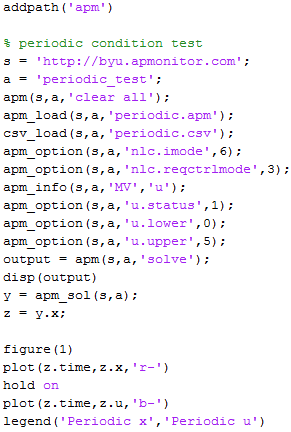
The following example illustrates the use of the boundary condition. Scripts in MATLAB and Python are available below to recreate this solution along with the model equations in APMonitor. Both MATLAB and Python scripts produce equivalent results.
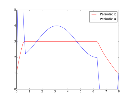
An example illustrates the use of periodic boundary conditions.
$$\min_u \left(x-3\right)^2$$
$$\frac{dx}{dt}+x=cos(t)+u$$
$$x(0)=x(8)=1$$
$$u(0)=u(8)=1$$
$$0 \le u \ge 5$$
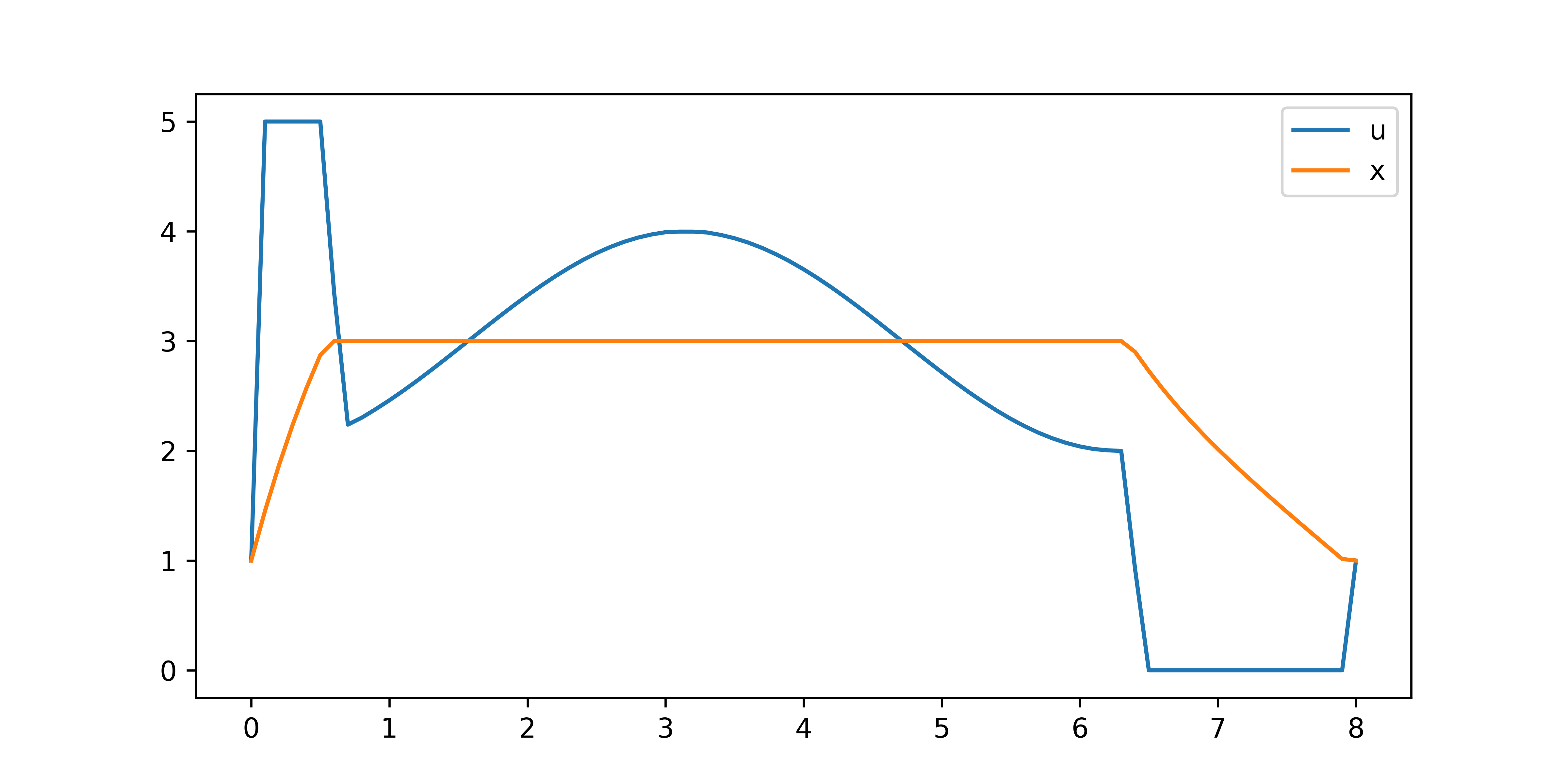
Scripts in MATLAB and Python are available below to recreate this solution along with the model equations in APMonitor. Both MATLAB and Python scripts produce equivalent results.

Periodic Example Script Files (periodic_example.zip)
APMonitor Model
(:toggle hide apmcode button show="Show APMonitor Model File":) (:div id=apmcode:)
(:toggle hide gkcode button show="Show GEKKO Python Source":) (:div id=gkcode:)
from gekko import GEKKO import numpy as np m = GEKKO() m.time = np.linspace(0,8,81) t = m.Param(m.time) u = m.MV(1,lb=0,ub=5); u.STATUS=1 x = m.Var(1) m.periodic(u) m.periodic(x) m.Minimize((x-3)**2) m.Equation(x.dt()+x==m.cos(t)+u) m.options.IMODE = 6 m.solve()
import matplotlib.pyplot as plt plt.plot(m.time,u,m.time,x) plt.legend(['u','x']) plt.show() (:sourceend:) (:divend:)
(:toggle hide apmcode button show="Show APMonitor Model File":) (:div id=apmcode:) (:source lang=python:)
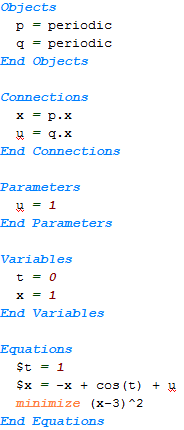
In the APMonitor software, boundary conditions are added for select variables with the use of a periodic object declaration.
Boundary conditions are added for select variables with the use of a periodic object declaration.
APMonitor Model
In Python Gekko, there is a periodic function.
In Python Gekko, there is a periodic function to add the APMonitor periodic condition.
Python Gekko
In the APMonitor software, boundary conditions are added for select variables with the use of a periodic object declaration. Linking this periodic object to a variable in the model enforces the periodic condition by adding an additional equation that the end point must be equal to the beginning point in the horizon.
In the APMonitor software, boundary conditions are added for select variables with the use of a periodic object declaration.
(:source lang=python:) Objects
q = periodic
End Objects (:sourceend:)
In Python Gekko, there is a periodic function.
(:source lang=python:) m.periodic(q) (:sourceend:)
Linking this periodic object to a variable in the model enforces the periodic condition by adding an additional equation that the end point must be equal to the beginning point in the horizon.
(:divend:)
(:toggle hide gekkocode button show="Show GEKKO Python Source":) (:div id=gekkocode:)
(:divend:)
(:source lang=matlab:)
(:toggle hide apmcode button show="Show APMonitor Model File":) (:div id=apmcode:) (:source lang=python:)
  vx >= 0 !used for energy storage representation
  vy >= 0	!used for energy recovery representation
  vx >= 0  # slack variable for energy storage representation
  vy >= 0  # slack variable for energy recovery representation
MATLAB Script
(:source lang=matlab:) Objects
q = periodic
End Objects
Connections
s = q.x
End Connections
Constants
eps = 0.7
End Constants
Parameters
  d
  p
End Parameters
Variables
  s >= 0 , = 100
  stored
  recovery
  vx >= 0 !used for energy storage representation
  vy >= 0	!used for energy recovery representation
End Variables
Equations
  minimize p
  p + recovery/eps - stored >= d
  p - d = vx- vy
  stored = p-d + vy
  recovery = d- p + vx
  $s = stored - recovery/ eps
  stored * recovery <= 0
End Equations
File *.plt
 New Trend
   p
   s
   d
End File (:sourceend:)
http://apmonitor.com/wiki/index.php/Apps/PeriodicBoundaryConditions
https://apmonitor.com/wiki/index.php/Apps/PeriodicBoundaryConditions
(:source lang=python:)
- !/usr/bin/env python3
- -*- coding: utf-8 -*-
""" Created on Mon Mar 8 21:34:49 2021
Gekko implementation of the simple energy storage model found here:
https://www.sciencedirect.com/science/article/abs/pii/S030626191500402X
Useful link:
http://apmonitor.com/wiki/index.php/Apps/PeriodicBoundaryConditions
@author: Nathaniel Gates, John Hedengren """
import numpy as np import matplotlib.pyplot as plt import matplotlib.ticker as mtick from gekko import GEKKO
m = GEKKO(remote=False)
t = np.linspace(0, 24, 24*3+1) m.time = t
m.options.SOLVER = 1 m.options.IMODE = 6 m.options.NODES = 3 m.options.CV_TYPE = 1 m.options.MAX_ITER = 300
p = m.FV() # production p.STATUS = 1 s = m.Var(100, lb=0) # storage inventory store = m.SV() # store energy rate vy = m.SV(lb=0) # store slack variable recover = m.SV() # recover energy rate vx = m.SV(lb=0) # recover slack variable
eps = 0.7
d = m.MV(-20*np.sin(np.pi*t/12)+100)
m.periodic(s)
m.Equations([p + recover/eps - store >= d,
             p - d == vx - vy,
             store == p - d + vy,
             recover == d - p + vx,
             s.dt() == store - recover/eps,
             store * recover <= 0])
m.Minimize(p)
m.solve(disp=True)
- Visualize results
fig, axes = plt.subplots(4, 1, sharex=True)
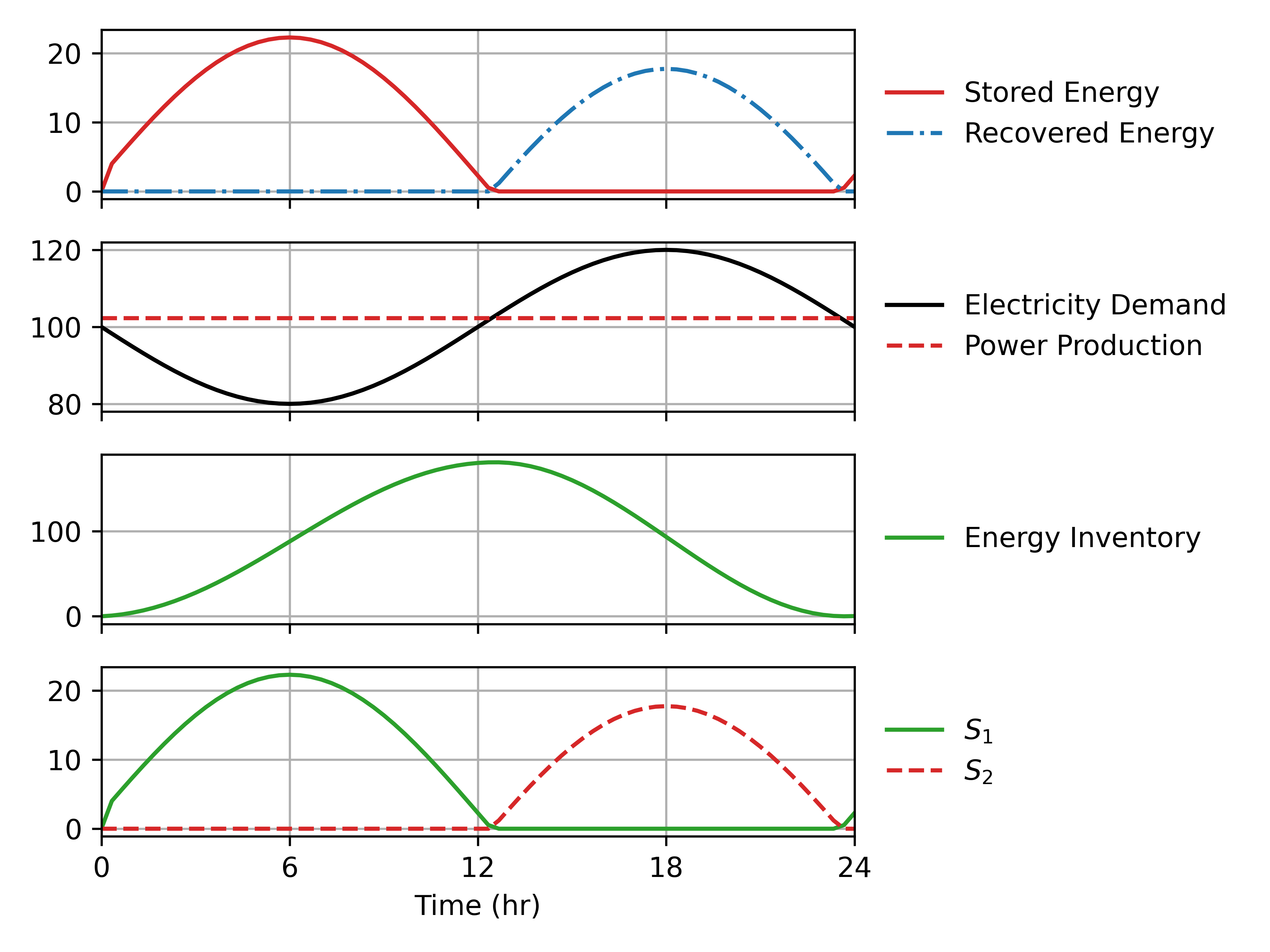
ax = axes[0] ax.plot(t, store, 'C3-', label='Store Rate') ax.plot(t, recover, 'C0-.', label='Recover Rate')
ax = axes[1] ax.plot(t, d, 'k-', label='Electricity Demand') ax.plot(t, p, 'C3--', label='Power Production')
ax = axes[2] ax.plot(t, s, 'C2-', label='Energy Inventory')
ax = axes[3] ax.plot(t, vx, 'C2-', label='$S_1$') ax.plot(t, vy, 'C3--', label='$S_2$') ax.set_xlabel('Time (hr)')
for ax in axes:
    ax.legend(bbox_to_anchor=(1.01, 0.5),               loc='center left', frameon=False)
    ax.grid()
    ax.set_xlim(0, 24)
    loc = mtick.MultipleLocator(base=6)
    ax.xaxis.set_major_locator(loc)
plt.tight_layout() plt.show() (:sourceend:)
Periodic Energy Storage in MATLAB/Python (periodic_energy_storage.zip)
The following example illustrates the use of the boundary condition. Scripts in MATLAB and Python are available below to recreate this solution.
The following example illustrates the use of the boundary condition. Scripts in MATLAB and Python are available below to recreate this solution along with the model equations in APMonitor. Both MATLAB and Python scripts produce equivalent results.
- MATLAB Script
APMonitor Model
MATLAB Script
- Python Script
Python Script
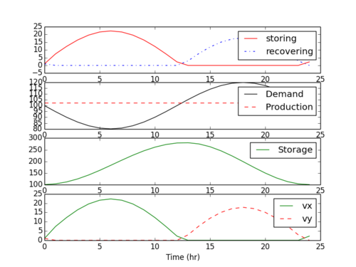
A further example demonstrates a more complicated model for energy storage and retrieval. In this case, energy is stored during the first hours of the day when demand is lower. The power generation runs at a constant level while the energy storage is able to follow the cyclical demand. Energy storage is set to a periodic boundary condition to ensure that the beginning and end of the day have at least 100 units of stored energy. Scripts are available in both MATLAB and Python.
Periodic Energy Storage Script Files (periodic_storage.zip) Δ
(:table border=1 width=100%:)
(:cell:) MATLAB
(:cell:) Python
(:cellnr:)
(:cell:) 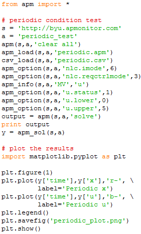 (:tableend:)
- MATLAB Script
- Python Script
(:title Periodic Boundary Conditions:) (:keywords periodic, Circadian rhythm, differential, algebraic, modeling language, numerical, boundary condition:) (:description Solve dynamic estimation and optimization problems with periodic boundary conditions.:)
Periodic boundary conditions arise in any situation where the end point must be equal to the beginning point. This type of boundary condition is typical where something is repeating many times but the optimization or simulation only needs to take place over one cycle of that sequence. An examples of a repeating process is the body's natural Circadian rhythm or a power plant that produces power to follow daily demand cycles. Examples of periodic boundary conditions in natural cycles or in manufacturing processes give importance to these conditions in numerical simulation.
In the APMonitor software, boundary conditions are added for select variables with the use of a periodic object declaration. Linking this periodic object to a variable in the model enforces the periodic condition by adding an additional equation that the end point must be equal to the beginning point in the horizon.
The following example illustrates the use of the boundary condition. Scripts in MATLAB and Python are available below to recreate this solution.
Periodic Example Script Files (periodic_example.zip)
(:table border=1 width=100%:)
(:cell:) MATLAB
(:cell:) Python
(:cellnr:)
(:cell:)
(:cell:)
(:tableend:)