High Index DAE Solution
Apps.PendulumMotion History
Hide minor edits - Show changes to markup
APMonitor and Gekko solve high index Differential and Algebraic Equations (DAEs) without rearrangement or differentiation. A common method for high index DAEs is to use Pantelides algorithm to reduce the index order. The index of a DAE is the number of times the equations must be differentiated to return to index-0 (ODE) form. Most ODE and DAE solvers have several challenges:
Solve high index Differential and Algebraic Equations (DAEs) without rearrangement or differentiation. A common method for high index DAEs is to use Pantelides algorithm to reduce the index order. The index of a DAE is the number of times the equations must be differentiated to return to index-0 (ODE) form. Most ODE and DAE solvers have several challenges:
(:html:) <iframe width="560" height="315" src="https://www.youtube.com/embed/Mj4OSUKHdXY" frameborder="0" allow="accelerometer; autoplay; clipboard-write; encrypted-media; gyroscope; picture-in-picture" allowfullscreen></iframe> (:htmlend:)
- Safdarnejad, S.M., Hedengren, J.D., Lewis, N.R., Haseltine, E., Initialization Strategies for Optimization of Dynamic Systems, Computers and Chemical Engineering, 2015, Vol. 78, pp. 39-50, DOI: 10.1016/j.compchemeng.2015.04.016 Article
- Safdarnejad, S.M., Hedengren, J.D., Lewis, N.R., Haseltine, E., Initialization Strategies for Optimization of Dynamic Systems, Computers and Chemical Engineering, 2015, Vol. 78, pp. 39-50, DOI: 10.1016/j.compchemeng.2015.04.016 Article
- Pendulum - Index 1 DAE
- Pendulum - Index 2 DAE
- Safdarnejad, S.M., Hedengren, J.D., Lewis, N.R., Haseltine, E., Initialization Strategies for Optimization of Dynamic Systems, Computers and Chemical Engineering, 2015, Vol. 78, pp. 39-50, DOI: 10.1016/j.compchemeng.2015.04.016. Article
- Safdarnejad, S.M., Hedengren, J.D., Lewis, N.R., Haseltine, E., Initialization Strategies for Optimization of Dynamic Systems, Computers and Chemical Engineering, 2015, Vol. 78, pp. 39-50, DOI: 10.1016/j.compchemeng.2015.04.016 Article
m \left( v^2 + w^2 - g \, y \right) - 2 \lambda \left( x^2 + y^2 \right) = 0
$$m \left( v^2 + w^2 - g \, y \right) - 2 \lambda \left( x^2 + y^2 \right) = 0$$
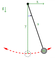
The pendulum weight is located on the end of a massless cord suspended from a pivot, without friction. When given an initial push, it swings back and forth at a constant amplitude. Real pendulums are subject to friction and air drag, so the amplitude of the swing declines.
A pendulum is used to investigate the effect of Differential and Algebraic (DAE) index with index-0 to index-3 DAE forms of the same model. The pendulum weight is located on the end of a massless cord suspended from a pivot, without friction. When given an initial push, it swings back and forth at a constant amplitude. Real pendulums are subject to friction and air drag, so the amplitude of the swing declines. The pendulum equations of motion calculate x-axis and y-axis positions as x and y and velocities as v and w, respectively. Additional parameters include m as the mass of pendulum, g as a gravitational constant, and s as the length of pendulum. The variable `\lambda` is a Lagrange multiplier.
A pendulum is used to investigate the effect of Differential and Algebraic (DAE) index with different forms of the same model. Index-0 to index-3 DAE forms are shown below with the simulation source code.
Index-0 DAE
$$\frac{d\lambda}{dt} = \frac{-4 \lambda \left( x \, v + y \, w \right) }{x^2+y^2}$$
Index-1 DAE
m \left( v^2 + w^2 - g \, y \right) - 2 \lambda \left( x^2 + y^2 \right) = 0
Index-2 DAE
$$x \, v + y \, w = 0$$
Index-3 DAE
$$x^2 + y^2 = s^2$$
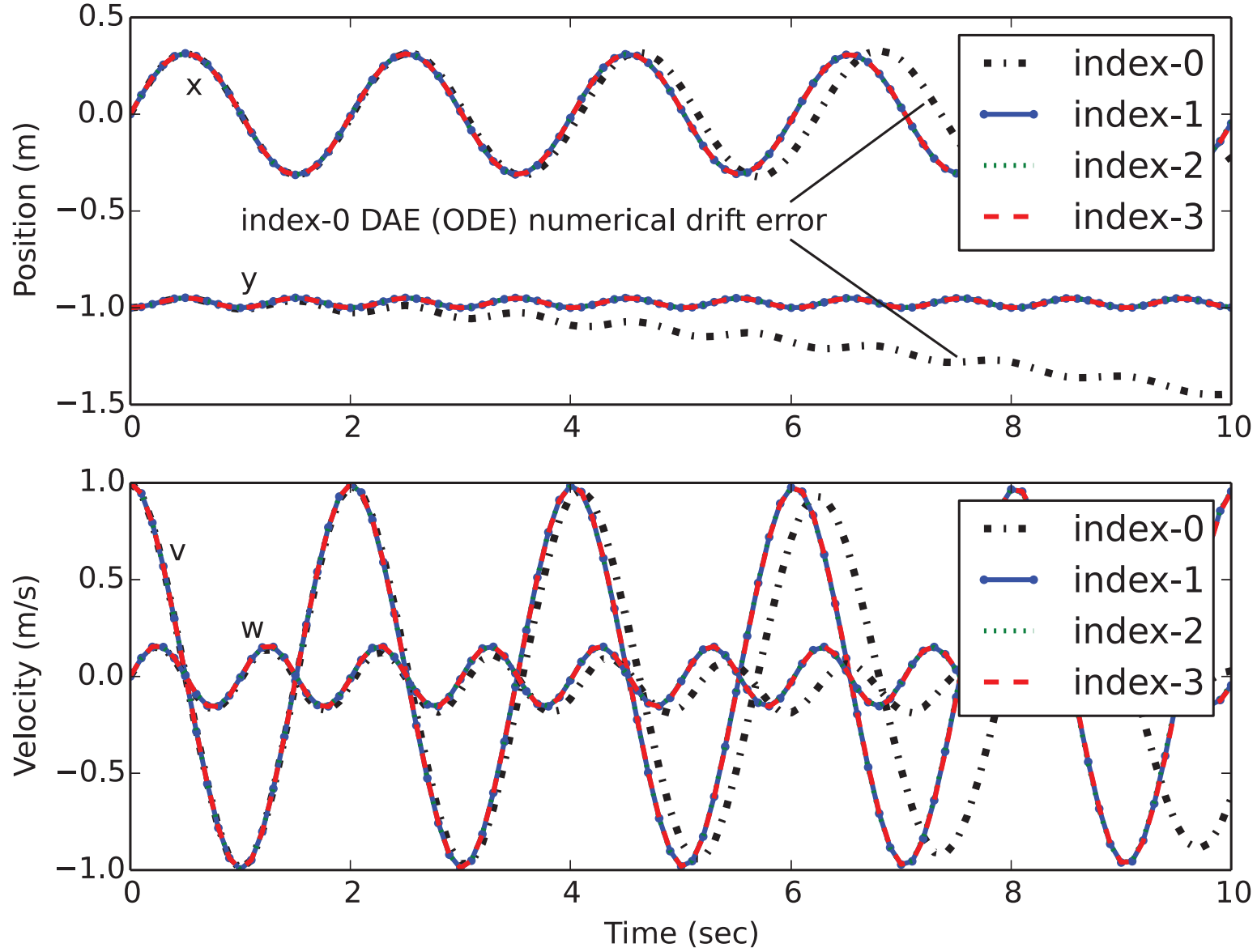
The following models are mathematically equivalent but are of different index order. The most natural form is an index-3 differential and algebraic (DAE) equation form, posed in terms of absolute position. The index is the number of times the equations must be differentiated to achieve an ordinary differential equation (ODE) form. This differentiation can cause numerical drift as seen in the
A pendulum is used to investigate the effect of Differential and Algebraic (DAE) index with different forms of the same model. Index-0 to index-3 DAE forms are shown below with the simulation source code.
The models are mathematically equivalent but are of different index order. The most natural form is an index-3 DAE equation form, posed in terms of absolute position. The index is the number of times the equations must be differentiated to achieve an ordinary differential equation (ODE) form. This differentiation can cause numerical drift as seen in the
See Inverted Pendulum Control and Crane Pendulum Modeling and Control
See Inverted Pendulum Control and Crane Pendulum Modeling and Control
References
- Safdarnejad, S.M., Hedengren, J.D., Lewis, N.R., Haseltine, E., Initialization Strategies for Optimization of Dynamic Systems, Computers and Chemical Engineering, 2015, Vol. 78, pp. 39-50, DOI: 10.1016/j.compchemeng.2015.04.016. Article
The following models are mathematically equivalent but are of different index order. The most natural form is an index-3 differential and algebraic (DAE) equation form, posed in terms of absolute position. The index is the number of times the equations must be differentiated to achieve an ordinary differential equation (ODE) form.
The following models are mathematically equivalent but are of different index order. The most natural form is an index-3 differential and algebraic (DAE) equation form, posed in terms of absolute position. The index is the number of times the equations must be differentiated to achieve an ordinary differential equation (ODE) form. This differentiation can cause numerical drift as seen in the
Predictions
The mass and length of a pendulum can be determined by tracking the horizontal position of the pendulum (x). The following is a MATLAB script (pendulum.m) that runs the Index-3 DAE through a series of simulations. As additional data is collected, the model predictions are adjusted to match the observed measurements. The starting values for mass are 1 kg and a length of 1 meter.
The technique for aligning measured and model values is termed Moving Horizon Estimation. This is a technique for parameter estimation with differential and algebraic equation models. In this case there is no steady state data available. The mass and length can be determined by observing the time series of horizontal positions.
(:html:)<font size=2><pre>
APMonitor Modeling Language
https://www.apmonitor.com
Pendulum - Index 3 DAE
Model pend3
  Parameters
    m = 1
    g = 9.81
    s = 1
  End Parameters

  Variables
    x = 0
    y = -s
    v = 1
    w = 0
    lam = m*(1+s*g)/2*s^2
  End Variables

  Equations
    x^2 + y^2 = s^2
    $x = v
    $y = w
    m*$v = -2*x*lam
    m*$w = -m*g - 2*y*lam
  End Equations
End Model </pre></font> (:htmlend:)
APMonitor and Gekko solve high index Differential and Algebraic Equations (DAEs) without rearrangement or differentiation. A common method for high index DAEs is to use Pantelides algorithm to reduce the index order. The index of a DAE is the number of times the equations must be differentiated to return to index-0 (ODE) form. This method has several challenges:
- A consistent initial condition is required
- Max index-1 or index-2 (Hessenberg form) is required
- There is numerical drift with repeated differentiation
APMonitor and Gekko solve high index Differential and Algebraic Equations (DAEs) without rearrangement or differentiation. A common method for high index DAEs is to use Pantelides algorithm to reduce the index order. The index of a DAE is the number of times the equations must be differentiated to return to index-0 (ODE) form. Most ODE and DAE solvers have several challenges:
- Consistent initial condition is required
- Required index-1 or index-2 (Hessenberg form)
- Numerical drift with repeated differentiation
APMonitor solves high index DAEs without differentiation with orthogonal collocation on finite elements and efficient solvers.
APMonitor and Gekko overcome these challenges by solving high index DAEs without differentiation with orthogonal collocation on finite elements and efficient sparse solvers.
(:description Solve high index DAEs with APMonitor and Gekko without algebraic rearrangement.:)
APMonitor and Gekko solve high index Differential and Algebraic Equations (DAEs) without rearrangement or differentiation. A common method for high index DAEs is to use Pantelides algorithm to reduce the index order. The index of a DAE is the number of times the equations must be differentiated to return to index-0 (ODE) form. APMonitor solves high index DAEs without differentiation with orthogonal collocation on finite elements and efficient solvers.
(:description Solve high index Differential Algebraic Equations (DAEs) in APMonitor and Gekko without consistent initial conditions, without differentiation of high index equations, and solution in the original form that does not have numerical drift.:)
APMonitor and Gekko solve high index Differential and Algebraic Equations (DAEs) without rearrangement or differentiation. A common method for high index DAEs is to use Pantelides algorithm to reduce the index order. The index of a DAE is the number of times the equations must be differentiated to return to index-0 (ODE) form. This method has several challenges:
- A consistent initial condition is required
- Max index-1 or index-2 (Hessenberg form) is required
- There is numerical drift with repeated differentiation
APMonitor solves high index DAEs without differentiation with orthogonal collocation on finite elements and efficient solvers.
Index-3 DAE Model
Predictions
The mass and length of a pendulum can be determined by tracking the horizontal position of the pendulum (x). The following is a MATLAB script (pendulum.m) that runs the Index-3 DAE through a series of simulations. As additional data is collected, the model predictions are adjusted to match the observed measurements. The starting values for mass are 1 kg and a length of 1 meter.
The technique for aligning measured and model values is termed Moving Horizon Estimation. This is a technique for parameter estimation with differential and algebraic equation models. In this case there is no steady state data available. The mass and length can be determined by observing the time series of horizontal positions.
(:html:)<font size=2><pre>
APMonitor Modeling Language
https://www.apmonitor.com
Pendulum - Index 3 DAE
Model pend3
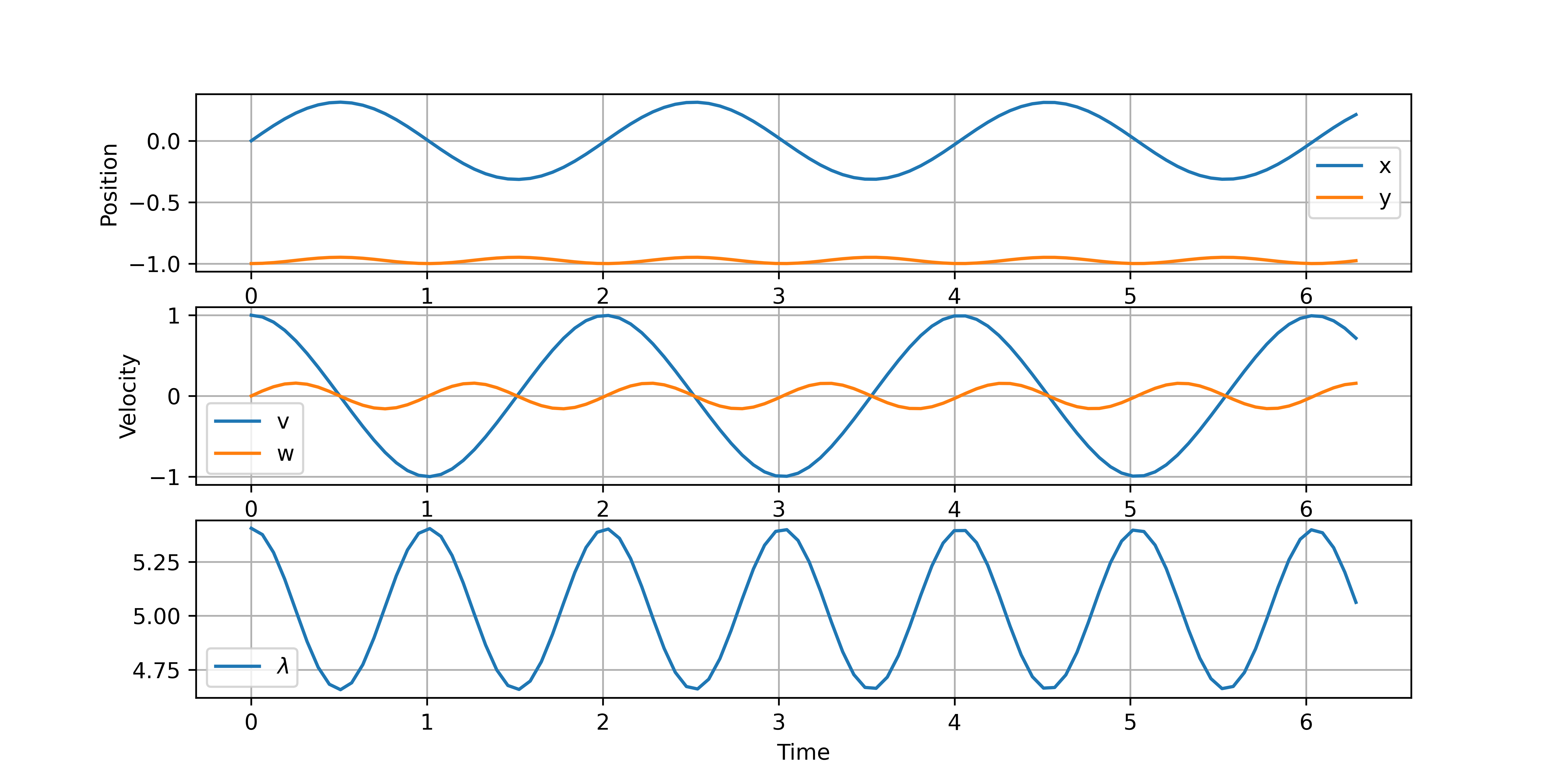
Some DAE numerical methods can solve up to index-2 DAEs in Hessenberg form. This is not required with Gekko and APMonitor that can solve any index-2 or higher DAE form. The index-2 form has no numerical drift but is still not as desirable as index-3 form that requires no rearrangement.
(:toggle hide gekko2 button show="Python Gekko Index-2 DAE":) (:div id=gekko2:) (:source lang=python:)
- Pendulum - Index 1 DAE
from gekko import GEKKO import numpy as np
mass = 1 g = 9.81 s = 1
m = GEKKO() x = m.Var(0) y = m.Var(-s) v = m.Var(1) w = m.Var(0) lam = m.Var(mass*(1+s*g)/2*s**2)
m.Equation(x*v + y*w==0) m.Equation(x.dt()==v) m.Equation(y.dt()==w) m.Equation(mass*v.dt()==-2*x*lam) m.Equation(mass*w.dt()==-mass*g-2*y*lam)
m.time = np.linspace(0,2*np.pi,100) m.options.IMODE=4 m.options.NODES=3 m.solve(disp=False)
import matplotlib.pyplot as plt plt.figure(figsize=(10,5)) plt.subplot(3,1,1) plt.plot(m.time,x.value,label='x') plt.plot(m.time,y.value,label='y') plt.ylabel('Position') plt.legend(); plt.grid() plt.subplot(3,1,2) plt.plot(m.time,v.value,label='v') plt.plot(m.time,w.value,label='w') plt.ylabel('Velocity') plt.legend(); plt.grid() plt.subplot(3,1,3) plt.plot(m.time,lam.value,label=r'$\lambda$') plt.legend(); plt.grid() plt.xlabel('Time') plt.savefig('index2.png',dpi=600) plt.show() (:sourceend:) (:divend:)
(:toggle hide apm2 button show="APMonitor Index-2 DAE":) (:div id=apm2:) (:source lang=fortran:)
Pendulum - Index 2 DAE
Model pend2
  Parameters
    m = 1
    g = 9.81
    s = 1
  End Parameters

  Variables
    x = 0
    y = -s
    v = 1
    w = 0
    lam = m*(1+s*g)/2*s^2
  End Variables

  Equations
    x * v + y * w = 0
    $x = v
    $y = w
    m*$v = -2*x*lam
    m*$w = -m*g - 2*y*lam
  End Equations
End Model (:sourceend:) (:divend:)
Index-3 DAE Model
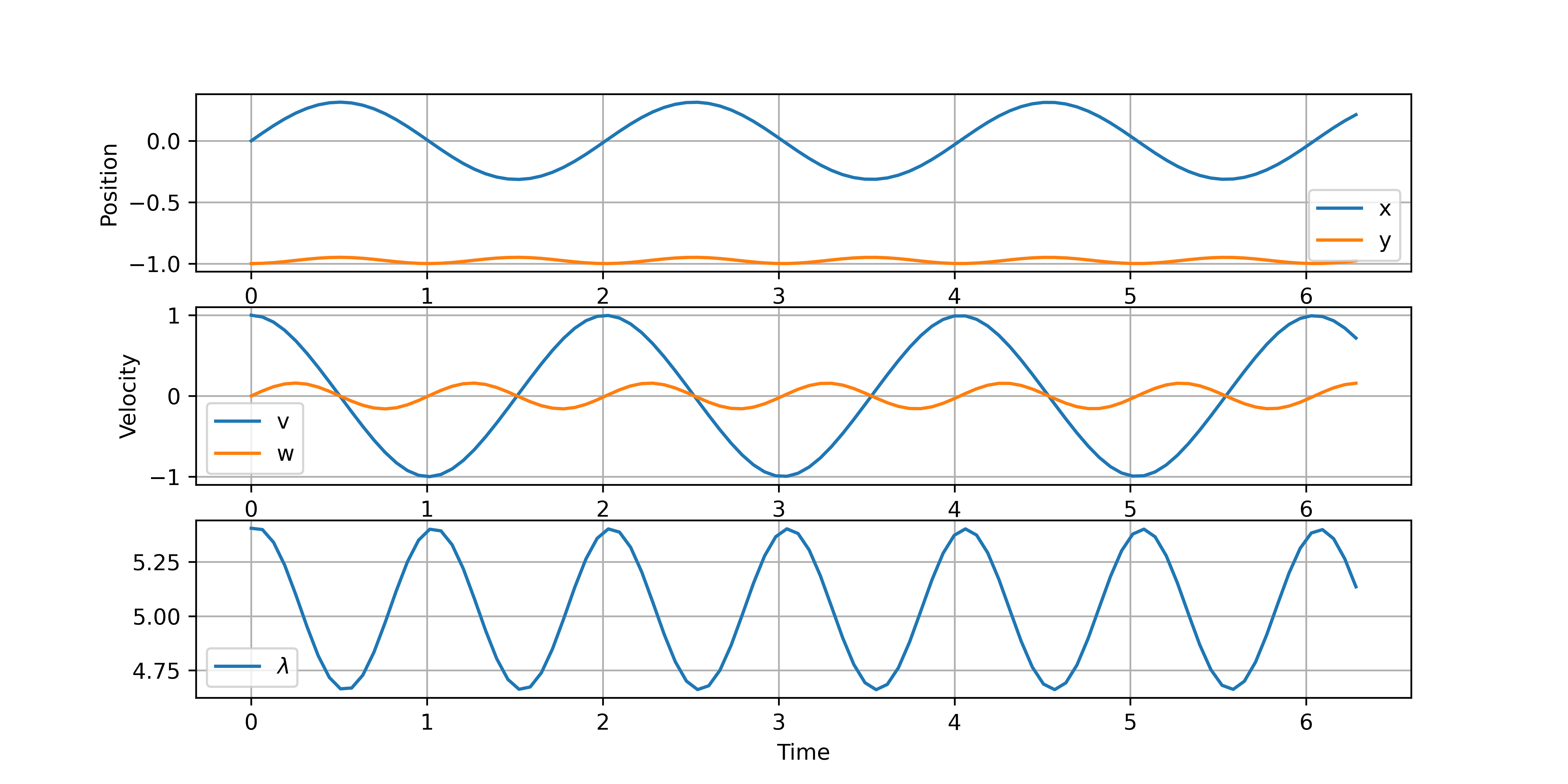
The index-3 form requires no rearrangement and has no numerical drift associated with index reduction. APMonitor and Gekko solve high-index DAEs with orthogonal collocation on finite elements either in simultaneous or sequential modes. This also allows the DAEs to be solved in optimization problems versus only simulation.

(:toggle hide gekko3 button show="Python Gekko Index-3 DAE":) (:div id=gekko3:) (:source lang=python:)
- Pendulum - Index 3 DAE
from gekko import GEKKO import numpy as np
mass = 1 g = 9.81 s = 1
m = GEKKO() x = m.Var(0) y = m.Var(-s) v = m.Var(1) w = m.Var(0) lam = m.Var(mass*(1+s*g)/2*s**2)
m.Equation(x**2+y**2==s**2) m.Equation(x.dt()==v) m.Equation(y.dt()==w) m.Equation(mass*v.dt()==-2*x*lam) m.Equation(mass*w.dt()==-mass*g-2*y*lam)
m.time = np.linspace(0,2*np.pi,100) m.options.IMODE=4 m.options.NODES=3 m.solve(disp=False)
import matplotlib.pyplot as plt plt.figure(figsize=(10,5)) plt.subplot(3,1,1) plt.plot(m.time,x.value,label='x') plt.plot(m.time,y.value,label='y') plt.ylabel('Position') plt.legend(); plt.grid() plt.subplot(3,1,2) plt.plot(m.time,v.value,label='v') plt.plot(m.time,w.value,label='w') plt.ylabel('Velocity') plt.legend(); plt.grid() plt.subplot(3,1,3) plt.plot(m.time,lam.value,label=r'$\lambda$') plt.legend(); plt.grid() plt.xlabel('Time') plt.savefig('index3.png',dpi=600) plt.show() (:sourceend:) (:divend:)
(:toggle hide apm3 button show="APMonitor Index-3 DAE":) (:div id=apm3:) (:source lang=fortran:)
Pendulum - Index 3 DAE
Model pend3
  Parameters
    m = 1
    g = 9.81
    s = 1
  End Parameters

  Variables
    x = 0
    y = -s
    v = 1
    w = 0
    lam = m*(1+s*g)/2*s^2
  End Variables

  Equations
    x^2 + y^2 = s^2
    $x = v
    $y = w
    m*$v = -2*x*lam
    m*$w = -m*g - 2*y*lam
  End Equations
End Model (:sourceend:) (:divend:)
plt.figure(figsize=(10,5))
plt.xlabel('Time') plt.savefig('index0.png',dpi=600)
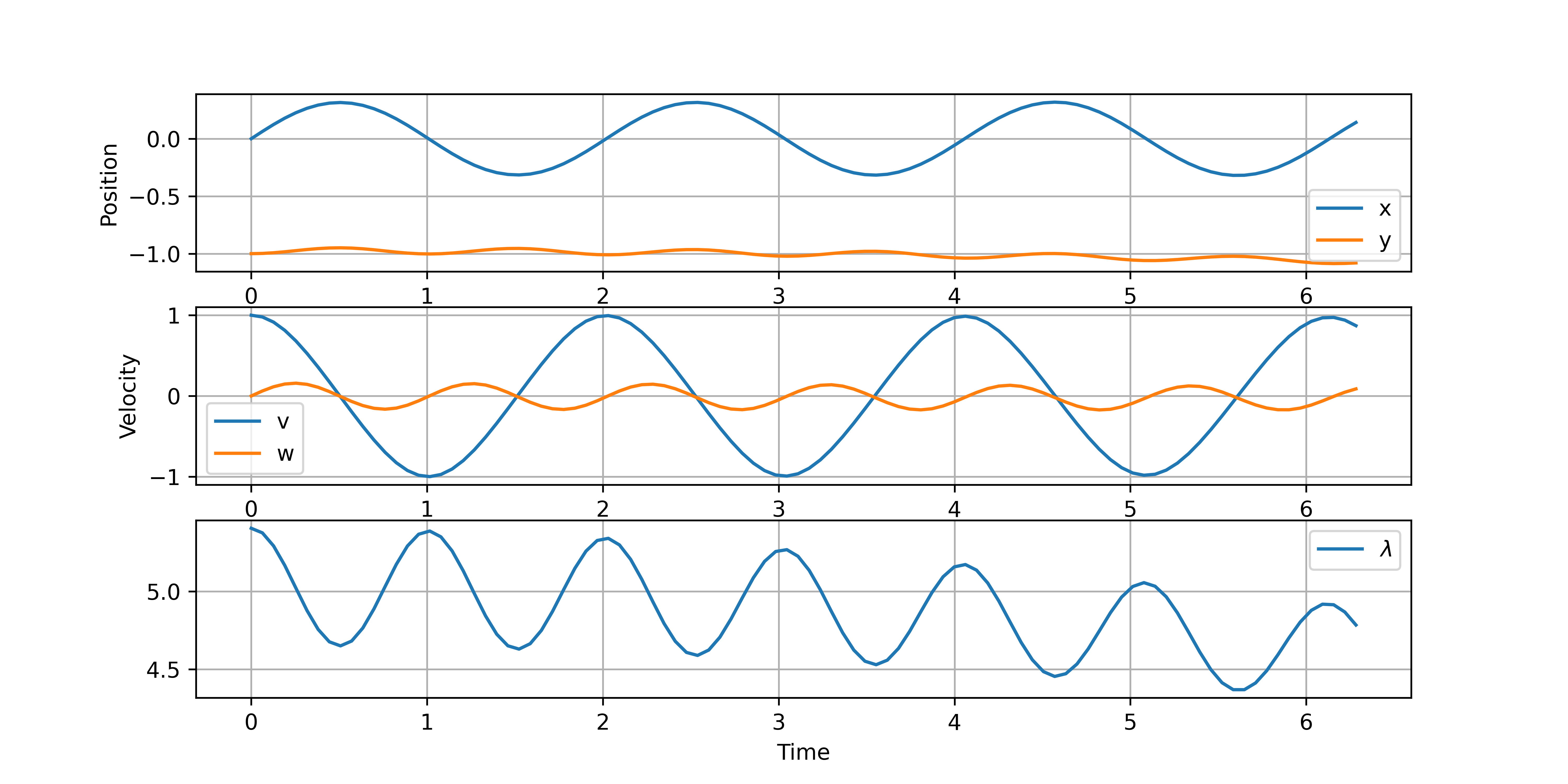
The differentiation of the equations (3 times) creates numerical drift in the solution, especially noticeable with lambda and y.
APMonitor Modeling Language
http://www.apmonitor.com
(:toggle hide apm1 button show="APMonitor Index-0 DAE":) (:div id=apm1:) (:source lang=matlab:)
(:sourceend:) (:divend:)
(:toggle hide gekko1 button show="Python Gekko Index-0 DAE":)
There is less numerical drift with the index-1 form but the solution is still not sufficiently accurate.
(:toggle hide gekko1 button show="Python Gekko Index-1 DAE":)
- Pendulum - Index 1 DAE
from gekko import GEKKO import numpy as np
mass = 1 g = 9.81 s = 1
m = GEKKO() x = m.Var(0) y = m.Var(-s) v = m.Var(1) w = m.Var(0) lam = m.Var(mass*(1+s*g)/2*s**2)
m.Equation(mass*(v**2+w**2-g*y)-2*lam*(x**2+y**2)==0) m.Equation(x.dt()==v) m.Equation(y.dt()==w) m.Equation(mass*v.dt()==-2*x*lam) m.Equation(mass*w.dt()==-mass*g - 2*y*lam)
m.time = np.linspace(0,2*np.pi,100) m.options.IMODE=4 m.options.NODES=3 m.solve(disp=False)
import matplotlib.pyplot as plt plt.figure(figsize=(10,5)) plt.subplot(3,1,1) plt.plot(m.time,x.value,label='x') plt.plot(m.time,y.value,label='y') plt.ylabel('Position') plt.legend(); plt.grid() plt.subplot(3,1,2) plt.plot(m.time,v.value,label='v') plt.plot(m.time,w.value,label='w') plt.ylabel('Velocity') plt.legend(); plt.grid() plt.subplot(3,1,3) plt.plot(m.time,lam.value,label=r'$\lambda$') plt.legend(); plt.grid() plt.xlabel('Time') plt.savefig('index1.png',dpi=600) plt.show() (:sourceend:) (:divend:)
(:toggle hide apm1 button show="APMonitor Index-1 DAE":) (:div id=apm1:) (:source lang=fortran:)
Pendulum - Index 1 DAE
Model pend1
  Parameters
    m = 1
    g = 9.81
    s = 1
  End Parameters

  Variables
    x = 0
    y = -s
    v = 1
    w = 0
    lam = m*(1+s*g)/2*s^2
  End Variables

  Equations
    m*(v^2+w^2-g*y) - 2*lam*(x^2+y^2) = 0
    $x = v
    $y = w
    m*$v = -2*x*lam
    m*$w = -m*g - 2*y*lam
  End Equations
End Model
(:source lang=matlab:)
(:source lang=fortran:)
(:toggle hide gekko0 button show="Python Gekko Index-0 DAE":) (:div id=gekko0:) (:source lang=python:)
- Pendulum - Index 0 DAE = ODE
from gekko import GEKKO import numpy as np
mass = 1 g = 9.81 s = 1
m = GEKKO() x = m.Var(0) y = m.Var(-s) v = m.Var(1) w = m.Var(0) lam = m.Var(mass*(1+s*g)/2*s**2)
m.Equation(lam.dt()==(-4*lam*(x*v+y*w) - 1.5*g*mass*w)/(x**2+y**2)) m.Equation(x.dt()==v) m.Equation(y.dt()==w) m.Equation(mass*v.dt()==-2*x*lam) m.Equation(mass*w.dt()==-mass*g - 2*y*lam)
m.time = np.linspace(0,2*np.pi,100) m.options.IMODE=4 m.options.NODES=3 m.solve(disp=False)
import matplotlib.pyplot as plt plt.subplot(3,1,1) plt.plot(m.time,x.value,label='x') plt.plot(m.time,y.value,label='y') plt.ylabel('Position') plt.legend(); plt.grid() plt.subplot(3,1,2) plt.plot(m.time,v.value,label='v') plt.plot(m.time,w.value,label='w') plt.ylabel('Velocity') plt.legend(); plt.grid() plt.subplot(3,1,3) plt.plot(m.time,lam.value,label=r'$\lambda$') plt.legend(); plt.grid() plt.show() (:sourceend:) (:divend:)
(:toggle hide apm0 button show="APMonitor Index-0 DAE":) (:div id=apm0:) (:source lang=matlab:)
APMonitor Modeling Language
http://www.apmonitor.com
Pendulum - Index 0 DAE = ODE
Model pend0
  Parameters
    m = 1
    g = 9.81
    s = 1
  End Parameters

  Variables
    x = 0
    y = -s
    v = 1
    w = 0
    lam = m*(1+s*g)/2*s^2
  End Variables

  Equations
    $lam = (-4*lam*(x*v+y*w) - 1.5*g*m*w)/(x^2+y^2)
    $x = v
    $y = w
    m*$v = -2*x*lam
    m*$w = -m*g - 2*y*lam
  End Equations
End Model (:sourceend:) (:divend:)
(:toggle hide apm1 button show="APMonitor Index-0 DAE":) (:div id=apm1:) (:source lang=matlab:)
(:sourceend:) (:divend:)
(:toggle hide gekko1 button show="Python Gekko Index-0 DAE":) (:div id=gekko1:) (:source lang=python:)
(:sourceend:) (:divend:)
(:title High Index DAE Solution:) (:keywords pendulum, Python, model, predictive control, APMonitor, differential, algebraic, modeling language:) (:description Solve high index DAEs with APMonitor and Gekko without algebraic rearrangement.:)
APMonitor and Gekko solve high index Differential and Algebraic Equations (DAEs) without rearrangement or differentiation. A common method for high index DAEs is to use Pantelides algorithm to reduce the index order. The index of a DAE is the number of times the equations must be differentiated to return to index-0 (ODE) form. APMonitor solves high index DAEs without differentiation with orthogonal collocation on finite elements and efficient solvers.
Index-0 to Index-3 Pendulum Example
- (:html:)<a href="/online/plot.php?d=pendulum&f=pend3.x.xml">Vertical Motion</a>(:htmlend:)
- (:html:)<a href="/online/plot.php?d=pendulum&f=pend3.y.xml">Horizontal Motion</a>(:htmlend:)
(:htmlend:)
(:htmlend:)
See Inverted Pendulum Control and Crane Pendulum Modeling and Control