Lecture Notes 33
Main.LectureNotes33 History
Hide minor edits - Show changes to markup
(:html:)
 <div id="disqus_thread"></div>
    <script type="text/javascript">
        /* * * CONFIGURATION VARIABLES: EDIT BEFORE PASTING INTO YOUR WEBPAGE * * */
        var disqus_shortname = 'apmonitor'; // required: replace example with your forum shortname

        /* * * DON'T EDIT BELOW THIS LINE * * */
        (function() {
            var dsq = document.createElement('script'); dsq.type = 'text/javascript'; dsq.async = true;
            dsq.src = 'https://' + disqus_shortname + '.disqus.com/embed.js';
            (document.getElementsByTagName('head')[0] || document.getElementsByTagName('body')[0]).appendChild(dsq);
        })();
    </script>
    <noscript>Please enable JavaScript to view the <a href="https://disqus.com/?ref_noscript">comments powered by Disqus.</a></noscript>
    <a href="https://disqus.com" class="dsq-brlink">comments powered by <span class="logo-disqus">Disqus</span></a>
(:htmlend:)
Homework
- Course reading for next class: None
- Assignment due by the start of Lecture #34: Work on Lab Projects
Relate each problem in the context of the overall course objectives.
<iframe width="560" height="315" src="//www.youtube.com/embed/YHAA-uXhI0E?list=PLLBUgWXdTBDgOlvGgbBDvHXdleSgEi9aj" frameborder="0" allowfullscreen></iframe>
<iframe width="560" height="315" src="//www.youtube.com/embed/YHAA-uXhI0E" frameborder="0" allowfullscreen></iframe>
<iframe width="560" height="315" src="//www.youtube.com/embed/YHAA-uXhI0E?list=UU2GuY-AxnNxIJFAVfEW0QFA" frameborder="0" allowfullscreen></iframe>
<iframe width="560" height="315" src="//www.youtube.com/embed/YHAA-uXhI0E?list=PLLBUgWXdTBDgOlvGgbBDvHXdleSgEi9aj" frameborder="0" allowfullscreen></iframe>
(:html:) <iframe width="560" height="315" src="//www.youtube.com/embed/YHAA-uXhI0E?list=UU2GuY-AxnNxIJFAVfEW0QFA" frameborder="0" allowfullscreen></iframe> (:htmlend:)
We use this example to develop an MPC application.
Model Predictive Control in Practice
(:html:) <iframe src="https://embed.ted.com/talks/raffaello_d_andrea_the_astounding_athletic_power_of_quadcopters.html" width="560" height="315" frameborder="0" scrolling="no" webkitAllowFullScreen mozallowfullscreen allowFullScreen></iframe> (:htmlend:)
Relate each problem in the context of the overall course objectives.
Relate each problem in the context of the overall course objectives.
(:html:)
 <div id="disqus_thread"></div>
    <script type="text/javascript">
        /* * * CONFIGURATION VARIABLES: EDIT BEFORE PASTING INTO YOUR WEBPAGE * * */
        var disqus_shortname = 'apmonitor'; // required: replace example with your forum shortname

        /* * * DON'T EDIT BELOW THIS LINE * * */
        (function() {
            var dsq = document.createElement('script'); dsq.type = 'text/javascript'; dsq.async = true;
            dsq.src = 'https://' + disqus_shortname + '.disqus.com/embed.js';
            (document.getElementsByTagName('head')[0] || document.getElementsByTagName('body')[0]).appendChild(dsq);
        })();
    </script>
    <noscript>Please enable JavaScript to view the <a href="https://disqus.com/?ref_noscript">comments powered by Disqus.</a></noscript>
    <a href="https://disqus.com" class="dsq-brlink">comments powered by <span class="logo-disqus">Disqus</span></a>
(:htmlend:)
Model Predictive Control (MPC) uses a mathematical representation of the process to predict and manipulate the future response of a system. Instead of a feedback strategy like PID control, MPC is actively making compensating moves to stay within constraints, drive to an economic optimum, and maximize or minimize certain quantities. Lecture 32 is an introduction to MPC and multivariable control.
Model Predictive Control (MPC) uses a mathematical representation of the process to predict and manipulate the future response of a system. Instead of a feedback strategy like PID control, MPC is actively making compensating moves to stay within constraints, drive to an economic optimum, and maximize or minimize certain quantities. Lecture 33 is an introduction to MPC and multivariable control.
MPC requires the numerical solution of dynamic equations. Below is a tutorial on solving differential and algebraic equations.
(:html:) <iframe width="560" height="315" src="https://www.youtube.com/embed/-IDTagajoyA" frameborder="0" allowfullscreen></iframe> (:htmlend:)
We use this example to develop an MPC application.
Optimization Review
As part of the review on optimization, homework problem 19.14 was covered in class.
Homework Problem 19.14 from Process Dynamics and Control (Seborg, Edgar, Mellichamp, Doyle)
A reversible chemical reaction, A->B and B->A, occurs in an isothermal continuous stirred-tank reactor. The rate expressions for the forward and reverse reactions are:
- r1 = k1 CA
- r2 = k2 CB
Using the information given below, use a numerical search procedure to determine the value of Fb (L/hr) that maximizes the production rate of Cb (i.e. the amount of Cb that leaves the reactor, mol B/hr). The allowable values of Fb are 0 <= Fb <= 200 L/hr.
Available information
- The reactor is perfectly mixed.
- The volume of liquid, V, is maintained constant using an overflow line (not shown in the diagram).
- The following parameters are kept constant at the indicated numerical values:
- V = 200 L
- FA = 150 L/hr
- CAF = 0.3 mol A/L
- CBF = 0.3 mol B/L
The solution to this problem is possible with a number of numerical or analytical techniques. One solution approach that we covered in class was with the APMonitor software through the web interface.
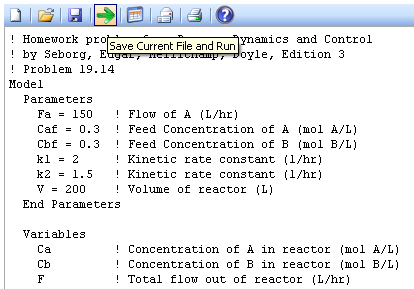
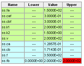
Equations and Solution to HW19.14
Equations for HW19.14

Solution to HW19.14

- Assignment due by the start of Lecture #34: None, Exam 3 is due Friday
- Assignment due by the start of Lecture #34: Work on Lab Projects
We'll also take some time to review material for closed-loop control analysis. This includes PID equations in the Laplace domain, stability analysis of proportional-only controllers, model predictive control, and optimization topics. A full listing of the topics are detailed in the attached worksheet.
We'll also take some time to review material for closed-loop control analysis. We formerly had an exam at this point in the semester but have replaced it with a second lab project. It is helpful to revisit the last couple weeks and get the big picture of where we are headed.
This review includes PID equations in the Laplace domain, stability analysis of proportional-only controllers, model predictive control, and optimization topics. A full listing of the topics are detailed in the attached worksheet.
Lecture 33 - Exam Review
Exam 3 covers material for closed-loop control analysis. This includes PID equations in the Laplace domain, stability analysis of proportional-only controllers, model predictive control, and optimization topics. A full listing of the topics are detailed in the attached worksheet.
Lecture 33 - Model Predictive Control
Model Predictive Control (MPC) uses a mathematical representation of the process to predict and manipulate the future response of a system. Instead of a feedback strategy like PID control, MPC is actively making compensating moves to stay within constraints, drive to an economic optimum, and maximize or minimize certain quantities. Lecture 32 is an introduction to MPC and multivariable control.
Course Review
We'll also take some time to review material for closed-loop control analysis. This includes PID equations in the Laplace domain, stability analysis of proportional-only controllers, model predictive control, and optimization topics. A full listing of the topics are detailed in the attached worksheet.
Equations for HW19.14
Solution to HW19.14
As part of the review on optimization, homework problem 19.14 was covered in class. This
Homework Problem 19.14
from Process Dynamics and Control (Seborg, Edgar, Mellichamp, Doyle)
Optimization Review
As part of the review on optimization, homework problem 19.14 was covered in class.
Homework Problem 19.14 from Process Dynamics and Control (Seborg, Edgar, Mellichamp, Doyle)
Homework Problem 19.14 from Process Dynamics and Control (Seborg, Edgar, Mellichamp, Doyle)
Homework Problem 19.14
from Process Dynamics and Control (Seborg, Edgar, Mellichamp, Doyle)
Lecture 33 - Exam Review
Exam 3 covers material for closed-loop control analysis. This includes PID equations in the Laplace domain, stability analysis of proportional-only controllers, model predictive control, and optimization topics. A full listing of the topics are detailed in the attached worksheet.
As part of the review on optimization, homework problem 19.14 was covered in class. This
Homework Problem 19.14 from Process Dynamics and Control (Seborg, Edgar, Mellichamp, Doyle)
A reversible chemical reaction, A->B and B->A, occurs in an isothermal continuous stirred-tank reactor. The rate expressions for the forward and reverse reactions are:
- r1 = k1 CA
- r2 = k2 CB
Using the information given below, use a numerical search procedure to determine the value of Fb (L/hr) that maximizes the production rate of Cb (i.e. the amount of Cb that leaves the reactor, mol B/hr). The allowable values of Fb are 0 <= Fb <= 200 L/hr.
Available information
- The reactor is perfectly mixed.
- The volume of liquid, V, is maintained constant using an overflow line (not shown in the diagram).
- The following parameters are kept constant at the indicated numerical values:
- V = 200 L
- FA = 150 L/hr
- CAF = 0.3 mol A/L
- CBF = 0.3 mol B/L
The solution to this problem is possible with a number of numerical or analytical techniques. One solution approach that we covered in class was with the APMonitor software through the web interface.
Equations and Solution to HW19.14
Homework
- Course reading for next class: None
- Assignment due by the start of Lecture #34: None, Exam 3 is due Friday
Relate each problem in the context of the overall course objectives.
