

Introduction to Engineering Optimization
Optimization Introduction in the Engineering Optimization online course.
Engineering optimization platforms in Python are an important tool for engineers in the modern world. They allow engineers to quickly and easily optimize complex engineering problems and tasks, such as design optimization, resource allocation, and route planning. This notebook has examples for solving LP, QP, NLP, MILP, and MINLP problems in Python.
- 1️⃣ Linear Programming (LP)
- 2️⃣ Quadratic Programming (QP)
- 3️⃣ Nonlinear Programming (NLP)
- 4️⃣ Mixed Integer Linear Programming (MILP)
- 5️⃣ Mixed Integer Nonlinear Programming (MINLP)
Install gekko Library
First, install the necessary gekko library for this notebook. The solutions to the examples are with scipy and gekko. Installing packages only needs to occur once and then it is always available in that Python distribution. Jupyter notebook may require a restart of the kernel to make the library accessible for import.
1️⃣ Linear Programming
A company manufactures two products (G and H) and has two resources (X and Y) available.
- Each unit of product G requires 3 units of resource X and 8 units of resource Y
- Each unit of product H requires 6 units of resource X and 4 units of resource Y
- The company has a maximum of 30 units of resource X and 44 units of resource Y available.
- The company wants to maximize profits:
- $100 per unit of product G
- $125 per unit of product H
Linear programming is an optimization method for solving systems of linear constraints and objectives. This problem is mathematically expressed as:
Maximize `100 G + 125 H`
Subject to:
$$3 G + 6 H <= 30$$
$$8 G + 4 H <= 44$$
$$G,H >= 0$$
where G and H are the number of units of products to be produced, respectively.
Scipy Linear Programming
The following code shows how to use linear programming to solve this problem in scipy.optimize with the linprog function. The linear programming problem is placed into the following matrix form:
$$\begin{align}\mathrm{minimize} \quad & c\,x \\ \mathrm{subject\;to}\quad & A \, x=b \\ & A_{ub} \, x<b_{ub} \end{align}$$
with:
$$x = [G,H]$$
$$c = [-4,-6]$$
$$A_{ub} = \begin{bmatrix}2 & 3\\ 1 & 1\end{bmatrix} \quad b_{ub}=[100,80]$$
c = [-100, -125]
A = [[3, 6], [8, 4]]
b = [30, 44]
bound = (0, None)
res = linprog(c, A_ub=A, b_ub=b, bounds=[bound, bound], method='highs')
#print solution
print(f'Optimal solution: G = {res.x[0]:.2f}, H = {res.x[1]:.2f}')
print(f'Maximum profit = $ {-res.fun:.2f}')
Gekko Linear Programming
The following code shows how to use linear programming to solve this problem in gekko. There is additional information on solving linear programming problems with sparse or dense matrices in gekko.

m = GEKKO()
G,H = m.Array(m.Var,2,lb=0)
m.Maximize(100*G+125*H)
m.Equation(3*G+6*H<=30)
m.Equation(8*G+4*H<=44)
m.solve(disp=False)
#print solution
print(f'Optimal solution: G = {G.value[0]:.2f}, H = {H.value[0]:.2f}')
print(f'Maximum profit = $ {-m.options.objfcnval:.2f}')
✅ Activity: Solve LP Problem
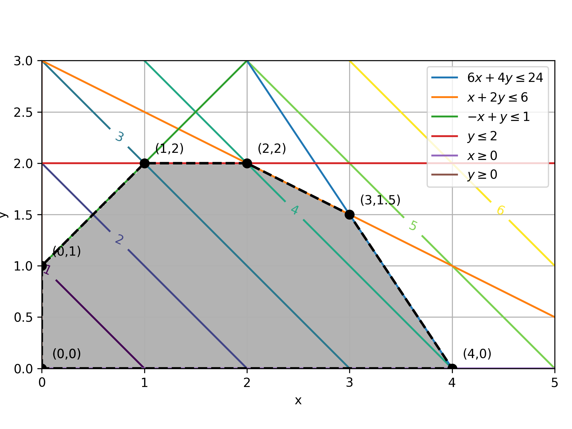
$$\begin{align}\mathrm{maximize} \quad & x+y \\ \mathrm{subject\;to}\quad & 6x+4y\le24 \\ & x+2y\le6 \\ &-x+y\le1 \\ & 0\le y\le2 \\ & x\ge0 \end{align}$$
Use either gekko or scipy to solve the LP and report the results for x, y, and the objective function value. Find the solution on the contour plot to graphically verify the results.
LP Solution Help
m = GEKKO(remote=False)
x,y = m.Array(m.Var,2,lb=0)
m.Equations([6*x+4*y<=24,x+2*y<=6,-x+y<=1,y<=2])
m.Maximize(x+y)
m.solve(disp=False)
xopt = x.value[0]; yopt = y.value[0]
print('x:', xopt,'y:', yopt,'obj:',-m.options.objfcnval)
Visualize Solution (Optional)
import matplotlib.pyplot as plt
#visualize solution
g = np.linspace(0,5,200)
x,y = np.meshgrid(g,g)
obj = x+y
plt.imshow(((6*x+4*y<=24)&(x+2*y<=6)&(-x+y<=1)&(y<=2)&(x>=0)&(y>=0)).astype(int),
extent=(x.min(),x.max(),y.min(),y.max()),origin='lower',cmap='Greys',alpha=0.3);
#plot constraints
x0 = np.linspace(0, 5, 2000)
y0 = 6-1.5*x0 # 6*x+4*y<=24
y1 = 3-0.5*x0 # x+2*y<=6
y2 = 1+x0 # -x+y<=1
y3 = (x0*0) + 2 # y <= 2
y4 = x0*0 # x >= 0
plt.plot(x0, y0, label=r'$6x+4y\leq24$')
plt.plot(x0, y1, label=r'$x+2y\leq6$')
plt.plot(x0, y2, label=r'$-x+y\leq1$')
plt.plot(x0, 2*np.ones_like(x0), label=r'$y\leq2$')
plt.plot(x0, y4, label=r'$x\geq0$')
plt.plot([0,0],[0,3], label=r'$y\geq0$')
xv = [0,0,1,2,3,4,0]; yv = [0,1,2,2,1.5,0,0]
plt.plot(xv,yv,'ko--',markersize=7,linewidth=2)
for i in range(len(xv)):
plt.text(xv[i]+0.1,yv[i]+0.1,f'({xv[i]},{yv[i]})')
#objective contours
CS = plt.contour(x,y,obj,np.arange(1,7))
plt.clabel(CS, inline=1, fontsize=10)
#optimal point
plt.plot([xopt],[yopt],marker='o',color='orange',markersize=10)
plt.xlim(0,5); plt.ylim(0,3); plt.grid(); plt.tight_layout()
plt.legend(loc=1); plt.xlabel('x'); plt.ylabel('y')
plt.show()
2️⃣ Quadratic Programming
A car manufacturer wants to minimize the weight of a car while maintaining a minimum strength requirement. The weight of the car is modeled as a quadratic function of the thickness of the car frame components. The strength of the car is modeled as a linear function of the thickness of the car frame components. The manufacturer wants to minimize the weight of the car while maintaining a minimum strength requirement. This problem is formulated as:
Minimize `\frac{1}{2} x^T Q x + p x`
Subject to:
$$G \, x >= h$$
where x is the thickness of the car frame components, Q is the quadratic weight coefficient matrix, p is the linear weight coefficient vector, G is the strength coefficient matrix, and h is the strength constraint vector.
#Quadratic weight coefficients
Q = np.array([[1, 0], [0, 2]])
#Linear weight coefficients
p = np.array([1, 2])
#Strength coefficients
G = np.array([[1, 1], [1, 2], [2, 1]])
#Strength constraints
h = np.array([3, 4, 5])
#Initial guess
x0 = np.array([0, 0])
Scipy Quadratic Programming
The minimize function in the scipy.optimize module is a general-purpose nonlinear optimization routine that can be used to find the minimum of a scalar function of one or more variables. To use it, you need to provide the following inputs:
constraints=con,bounds=bnds,
method='SLSQP',options=opt)
- Objective function: This should be a Python function that has decision variables as inputs and returns a scalar value to be minimized.
- The initial guess for the variables: This should be an array of initial guesses for the variables.
- Constraints with any inequality and equality bounds in residual format.
- Bounds: upper and lower bounds on the decision variables.
- Method: This is an optional parameter that specifies the optimization algorithm.
- Options: Configure parameters for solving the optimization problem.
#Define objective function
def objective_function(x):
return 0.5 * x @ Q @ x + p @ x
#Define constraints
def constraint(x):
return G @ x - h
#Define optimization
con = {'type': 'ineq', 'fun': constraint}
b = (0,10); bnds = (b,b)
opt = {'maxiter':1000}
res = minimize(objective_function, x0,
constraints=con,bounds=bnds,
method='SLSQP',options=opt)
#print results
print(f'Optimal solution: x = {res.x}')
print(f'Minimum weight = {res.fun}')
Gekko Quadratic Programming
The following code shows how to use quadratic programming in gekko. Change to remote=False to solve locally instead of using the public compute server. The public server has additional solver options.
x = m.Array(m.Var,2,lb=0,ub=10)
m.Minimize(0.5 * x@Q@x + p@x)
gx = G@x
m.Equations([gx[i]>=h[i] for i in range(len(h))])
m.solve(disp=False)
#print results
print(f'Optimal solution: x = {x}')
print(f'Minimum weight = {m.options.objfcnval}')
✅ Activity: Solve QP Problem
$$\begin{align}\mathrm{maximize} \quad & \frac{1}{2} \left(x^2+y^2\right) -2x+2y \\ \mathrm{subject\;to}\quad & 6x+4y\le24 \\ & x+2y\le6 \\ &-x+y\le1 \\ & 0\le y\le2 \\ & x\ge0 \end{align}$$
Use either gekko or scipy to solve the QP and report the results for x, y, and the objective function value.
Visualize QP Objective and Constraints
g = np.linspace(0,5,200)
x,y = np.meshgrid(g,g)
obj = 0.5*(x**2+y**2)-2*x+2*y
plt.imshow(((6*x+4*y<=24)&(x+2*y<=6)&(-x+y<=1)&(y<=2)&(x>=0)&(y>=0)).astype(int),
extent=(x.min(),x.max(),y.min(),y.max()),origin='lower',cmap='Greys',alpha=0.3);
#plot constraints
x0 = np.linspace(0, 5, 2000)
y0 = 6-1.5*x0 # 6*x+4*y<=24
y1 = 3-0.5*x0 # x+2*y<=6
y2 = 1+x0 # -x+y<=1
y3 = (x0*0) + 2 # y <= 2
y4 = x0*0 # x >= 0
plt.plot(x0, y0, label=r'$6x+4y\leq24$')
plt.plot(x0, y1, label=r'$x+2y\leq6$')
plt.plot(x0, y2, label=r'$-x+y\leq1$')
plt.plot(x0, 2*np.ones_like(x0), label=r'$y\leq2$')
plt.plot(x0, y4, label=r'$x\geq0$')
plt.plot([0,0],[0,3], label=r'$y\geq0$')
xv = [0,0,1,2,3,4,0]; yv = [0,1,2,2,1.5,0,0]
plt.plot(xv,yv,'ko--',markersize=7,linewidth=2)
for i in range(len(xv)):
plt.text(xv[i]+0.1,yv[i]+0.1,f'({xv[i]},{yv[i]})')
#objective contours
CS = plt.contour(x,y,obj,np.arange(1,7))
plt.clabel(CS, inline=1, fontsize=10)
plt.xlim(0,5); plt.ylim(0,3); plt.grid(); plt.tight_layout()
plt.legend(loc=1); plt.xlabel('x'); plt.ylabel('y')
plt.show()
QP Solution Help
m = GEKKO(remote=False)
x,y = m.Array(m.Var,2,lb=0)
m.Equations([6*x+4*y<=24,x+2*y<=6,-x+y<=1,y<=2])
m.Maximize(0.5*(x**2+y**2)-2*x+2*y)
m.solve(disp=False)
xopt = x.value[0]; yopt = y.value[0]
print('x:', xopt,'y:', yopt,'obj:',-m.options.objfcnval)
3️⃣ Nonlinear Programming
A nonlinear optimization problem is the Hock Schittkowski problem 71.
$$\min x_0 x_3 \left(x_0 + x_1 + x_2\right) + x_2$$
$$\mathrm{s.t.} \quad x_0 x_1 x_2 x_3 \ge 25$$
$$x_0^2 + x_1^2 + x_2^2 + x_3^2 = 40$$
$$1\le x \le 5$$
$$x_{init} = (1,5,5,1)$$
This problem has a nonlinear objective that must be minimized. The variable values at the optimal solution are subject to (s.t.) both equality (=40) and inequality (>=25) constraints. The product of the four variables must be greater than 25 while the sum of squares of the variables must also equal 40. In addition, all variables are constrained between 1 and 5 and the initial guess is x=[1,5,5,1].
Scipy Nonlinear Programming
def objective(x):
return x[0]*x[3]*(x[0]+x[1]+x[2])+x[2]
def constraint1(x):
return x[0]*x[1]*x[2]*x[3]-25.0
def constraint2(x):
sum_eq = 40.0
for i in range(4):
sum_eq = sum_eq - x[i]**2
return sum_eq
#initial guesses
x0 = [1,5,5,1]
#optimize
b = (1.0,5.0)
bnds = (b, b, b, b)
con1 = {'type': 'ineq', 'fun': constraint1}
con2 = {'type': 'eq', 'fun': constraint2}
cons = ([con1,con2])
solution = minimize(objective,x0,method='SLSQP',\
bounds=bnds,constraints=cons)
x = solution.x
#print solution
print('Objective: ' + str(objective(x)))
print('Solution:',x)
Gekko Nonlinear Programming
The following code shows how to solve nonlinear programming problems in gekko. All solvers in gekko can solve LP, QP, and NLP problems.
import numpy as np
m = GEKKO(remote=False)
x = m.Array(m.Var,4,value=1,lb=1,ub=5)
x1,x2,x3,x4 = x
#change initial values
x2.value = 5; x3.value = 5
m.Equation(x1*x2*x3*x4>=25)
m.Equation(x1**2+x2**2+x3**2+x4**2==40)
m.Minimize(x1*x4*(x1+x2+x3)+x3)
m.solve(disp=False)
#print solution
print('Objective: ',m.options.OBJFCNVAL)
print('Solution: ', x)
✅ Activity: Solve NLP Problem
$$\begin{align}\mathrm{minimize} \quad & xy^2-x^2-y^2 \\ \mathrm{subject\;to}\quad & x+y\ge4 \\ & xy<=5 \\ & 1\le x\le3 \\ & 2\le y\le3 \end{align}$$
Use either gekko or scipy to solve the NLP and report the results for x, y, and the objective function value.
Visualize NLP Objective and Constraints
g = np.linspace(1,3,200)
h = np.linspace(2,3,200)
x,y = np.meshgrid(g,h)
obj = x*y**2-x**2-y**2
plt.imshow(((x+y>=4)&(x*y<=5)&(x>=0)&(y>=0)).astype(int),
extent=(x.min(),x.max(),y.min(),y.max()),origin='lower',cmap='Greys',alpha=0.3);
#plot constraints
x0 = np.linspace(1,3,2000)
y0 = 4-x0 # x+y>=4
y1 = 5.0/x0 # x*y<=5
plt.plot(x0,y0,':',color='orange',linewidth=2,label=r'$x+y\geq4$')
plt.plot(x0,y1,'k--',linewidth=2,label=r'$xyleq5$')
plt.plot([1,1],[2,3],'b-',label=r'$x\geq1$')
plt.plot([3,3],[2,3],'b:',label=r'$x\leq3$')
plt.plot([1,3],[2,2],'k-',label=r'$y\geq2$')
plt.plot(x0, 3*np.ones_like(x0),'k:',label=r'$y\leq3$')
#objective contours
CS = plt.contour(x,y,obj,np.round(np.linspace(0,10,21),1))
plt.clabel(CS, inline=1, fontsize=10)
plt.xlim(0.9,3.1); plt.ylim(1.9,3.1); plt.grid(); plt.tight_layout()
plt.legend(loc=1); plt.xlabel('x'); plt.ylabel('y')
plt.show()
NLP Solution Help
m = GEKKO(remote=False)
x,y = m.Array(m.Var,2,lb=1,ub=3)
y.LOWER=2
m.Minimize(x*y**2-x**2-y**2)
m.Equations([x+y>=4,x*y<=5])
m.solve(disp=False)
xopt = x.value[0]; yopt = y.value[0]
print('x:', xopt,'y:', yopt,'obj:',-m.options.objfcnval)
4️⃣ Mixed Integer Linear Programming
Mixed integer linear programming (MILP) is a type of optimization problem that involves both continuous and discrete (integer) variables. In contrast, regular linear programming (LP) only involves continuous variables. The presence of integer variables in MIP makes the problem more difficult to solve, as the solution space is now discrete rather than continuous. This means that many of the techniques used for solving LP problems are not applicable to MIP. Specialized algorithms and solvers, such as branch-and-bound and branch-and-cut, are typically used to solve MIP problems.
Scipy Mixed Integer Linear Programming
Use the integrality option in the linprog function to specify:
- 0: continuous
- 1: integer
#Define the objective function
c = [-1, 4] # minimize -x + 4y
#Define the constraints
A_u = np.array([[3, 2], [1, 5]])
b_u = np.array([10,10])
#Define the bounds
b = (0, 10) # 0 <= x <= 10
#Solve
res = linprog(c, A_ub=A_u, b_ub=b_u, bounds=(b,b),
integrality=[1,1])
#Print the results
print("Objective function: ", res.fun)
print("Optimal solution: ", res.x)
Gekko Mixed Integer Linear Programming
The following code shows how to solve mixed integer linear programming problems. Use integer=True to specify an integer variable. The solver APOPT is a mixed integer solver in gekko that is selected with m.options.SOLVER=1.
x = m.Array(m.Var,2,lb=0,ub=10,integer=True)
m.Minimize(c@x)
Ax = A_u@x
m.Equations([Ax[i]<=b_u[i] for i in range(len(b_u))])
m.options.SOLVER=1
m.solve(disp=False)
#Print the results
print("Objective function: ", m.options.objfcnval)
print("Optimal solution: ", x)
✅ Activity: Solve an MILP Problem
$$\begin{align}\mathrm{maximize} \quad & x+y \\ \mathrm{subject\;to}\quad & 6x+4y\le24 \\ & x+2y\le6 \\ &-x+y\le1 \\ & 0\le y\le2 \\ & x\ge0 \end{align}$$
where x and y are integer values. Use either gekko or scipy to solve the MILP and report the results for x, y, and the objective function value. There are 3 potential solutions. Find the integer solutions on the contour plot to graphically verify the results.
MILP Solution Help
m = GEKKO(remote=False)
x,y = m.Array(m.Var,2,lb=0,integer=True)
m.Equations([6*x+4*y<=24,x+2*y<=6,-x+y<=1,y<=2])
m.Maximize(x+y)
m.solve(disp=False)
xopt = x.value[0]; yopt = y.value[0]
print('x:', xopt,'y:', yopt,'obj:',-m.options.objfcnval)
5️⃣ Mixed Integer Nonlinear Programming
Mixed integer nonlinear programming (MINLP) is like MILP but may have a nonlinear objective and constraints. It also requires specialized solvers such as the APOPT solver in gekko. There is no current MINLP solver for scipy, but that is likely changing in a future release.
m = GEKKO() # create GEKKO model
#create integer variables
x1 = m.Var(integer=True,lb=-5,ub=10)
x2 = m.Var(integer=True,lb=-1,ub=2)
#create continuous variable
x3 = m.Var(lb=0)
m.Minimize(4*x1**2-4*x2*x1**2+x2**2+x1**2-x1+x3**2)
m.Equation(x3*x2>=1)
m.options.SOLVER = 1 # APOPT solver
m.solve(disp=False)
print('x1: ' + str(x1.value[0]))
print('x2: ' + str(x2.value[0]))
print('x3: ' + str(x3.value[0]))
In addition to binary (0,1) and integer variables, Special Ordered Sets are also possible to define from a selection of discrete options such as [0.5, 1.15, 2.6, 5.2].
m = GEKKO() # create GEKKO model
#integer variable
x1 = m.Var(integer=True,lb=-5,ub=10)
#create Special Ordered Set variable
x2 = m.sos1([0.5, 1.15, 2.6, 5.2])
#continuous variable
x3 = m.Var(lb=0)
m.Minimize(4*x1**2-4*x2*x1**2+x2**2+x1**2-x1+x3**2)
m.Equation(x3*x2>=1)
m.options.SOLVER = 1 # APOPT solver
m.solve(disp=False)
print('x1: ' + str(x1.value[0]))
print('x2: ' + str(x2.value[0]))
print('x3: ' + str(x3.value[0]))
✅ Activity: Solve MINLP Problem
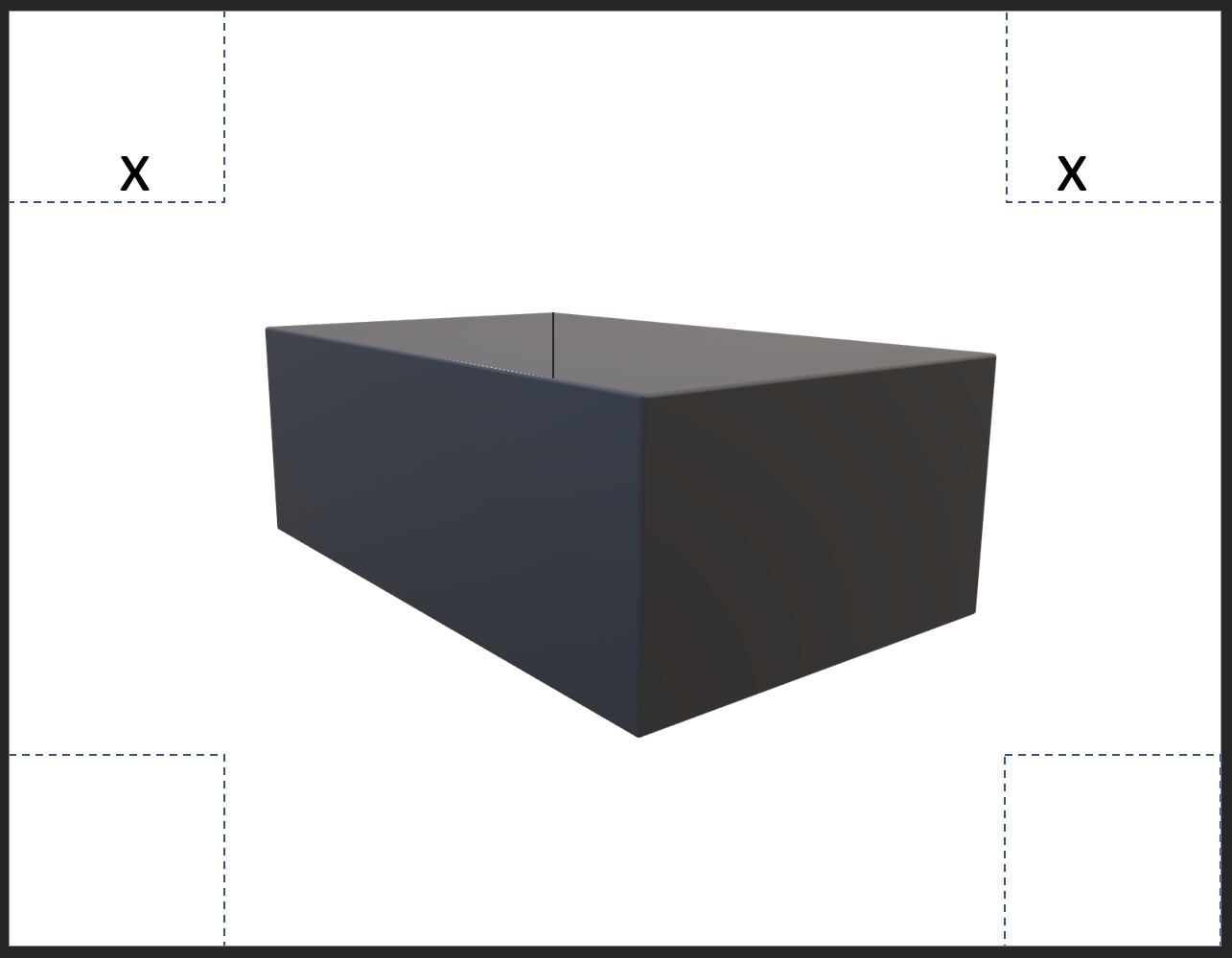
A piece of letter paper 8.5x11 inches is made into an open-top box by first removing the corners and then by folding the sides up to the adjacent side. The starting sheet has height and width. The objective is to maximize the volume of the box (no lid) by choosing an appropriate value of x (the height of the box).
- Print a Box Folding Template (PDF)
- Additional information on paper box folding with solution help.
Starting with the continuous solution, restrict the height to inch values in integer increments. Below is the continuous solution:
m = GEKKO(remote=False)
paper_width = 8.5 # width of paper
paper_length = 11 # length of paper
x = m.Var(lb=0) # cut out length
box_width = m.Intermediate(paper_width - 2 * x)
box_length = m.Intermediate(paper_length - 2 * x)
box_height = m.Intermediate(x)
Volume = m.Intermediate(box_width * box_length * box_height)
#lower constraint for box width with tabs
m.Equations([box_width > 0,box_length > 0,Volume > 0.01])
m.Maximize(Volume)
m.options.SOLVER=1
m.solve(disp=False)
print('width = ' + str(box_width.value[0]))
print('length = ' + str(box_length.value[0]))
print('height = ' + str(box_height.value[0]))
print('volume = ' + str(Volume.value[0]))
Calculate how much the integer solution requirement decreases the volume.
Python Gekko Examples
These tutorial are examples of using Python Gekko to solve an optimization problem.