Logical Conditions in Optimization

Conditional statements can cause problems for gradient-based optimization algorithms because they are often posed in a form that gives discontinuous functions, first derivatives, or second derivatives.

For example, the absolute value operator is a continuous function but gives a discontinuous first derivative at the origin.

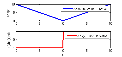
Minimizing this function can cause a problem for solvers that rely on first and second derivative information to determine search directions at each iteration. As an exercise, solve the following model that uses the absolute value operator.

• Example 1: Absolute Value Operator Away from the Discontinuity

The solver can still converge because the solution is away from the discontinuity. In Example 2, the value of x is now determined by the optimizer. The objective function to minimize (y+3)² means that the optimal solution is at x=0 and y=0. However, when the solution is at the discontinuity, a gradient based solver will often fail to converge.

• Example 2: Absolute Value Operator at the Discontinuity

In this case, the IPOPT solver reaches the default maximum number of iterations (100) and reports a failure to converge. However, if another form with continuous first and second derivatives (abs2 in GEKKO) is used, a solution is found.

Also, if the problem is reformulated with an additional binary variable intb, the optimizer can find a solution to the same problem that failed with the abs(x) operator. The value of intb is a binary variable that can be either 0 or 1. The value of intb is zero when x<0 and is one when x>=0. The following two examples show that this reformulation allows the solver to quickly find a solution either away from or at the discontinuity.

• Example 3: Absolute Value away from the Discontinuity

• Example 4: Absolute Value at the Discontinuity

The above examples demonstrate this concept with the absolute value operator. The same techniques can be applied to:

• If...Else Statements
• Max Function (see Python GEKKO max2 and max3 functions)
• Min Function (see Python GEKKO min2 and min3 functions)
• Minimax and Maximin
• Piece-wise Linear Functions (see Python GEKKO pwl function)
• Signum Function (What is Signum?)
• Other discontinuous functions

import numpy as np
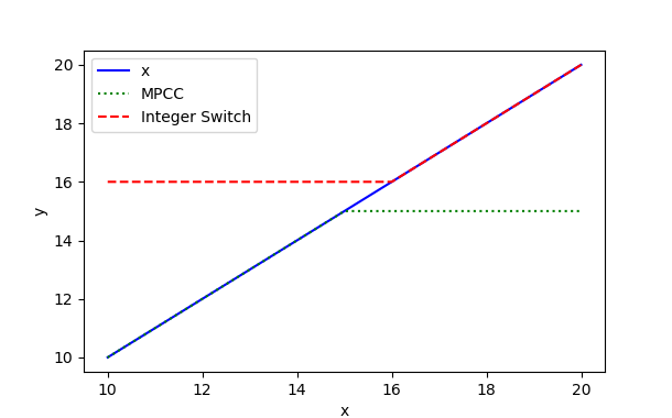
import matplotlib.pyplot as plt
from gekko import GEKKO
m = GEKKO(remote=False)
p = m.Param(value=np.linspace(10,20,21))
x = m.Var()
m.Equation(x==p)
# with MPCCs
y2 = m.min2(p,15)
# with integer variables
y3 = m.max3(p,16)
m.options.IMODE = 2
m.solve()
plt.plot(p,x,'b-',label='x')
plt.plot(p,y2,'g:',label='MPCC')
plt.plot(p,y3,'r--',label='Integer Switch')
plt.legend()
plt.xlabel('x')
plt.ylabel('y')
plt.show()

[$[Get Code]]

import numpy as np
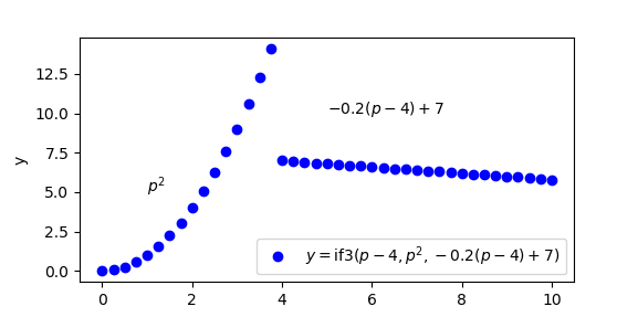
import matplotlib.pyplot as plt
from gekko import GEKKO
m = GEKKO(remote=False)
p = m.Param(value=np.linspace(0,10,41))
# conditional statement
y = m.if3(p-4,p**2,-0.2*(p-4)+7)
m.options.IMODE = 2
m.solve()
lbl = r'$y=\mathrm{if3}(p-4,p^2,-0.2(p-4)+7)$'
plt.plot(p,y,'bo',label=lbl)
plt.text(1,5,r'$p^2$')
plt.text(5,10,r'$-0.2 (p-4)+7$')
plt.legend(loc=4)
plt.ylabel('y')
plt.show()

[$[Get Code]]

Two popular methods for reformulation of the conditional statements is to either use:

• Binary or integer variables
• Mathematical Programs with Equilibrium/Complementarity Constraints (MPECs/MPCCs)

Each of these techniques are described below with a number of examples.

Logical Conditions with Binary Variables

The approach taken above with the ABS function used a single binary variable.

• ABS: Absolute Value Operator (Integer Form)

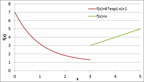
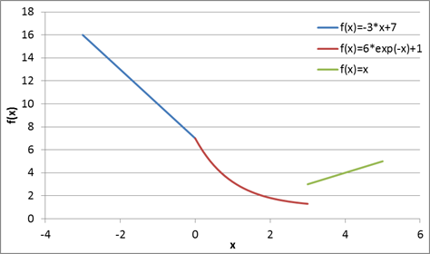
The following examples demonstrate the use of conditional statements to switch between different functions. In this case, the function y=6*exp(-x)+1 if the value of x<3 else the function y=x is chosen when x>=3. The simulate example verifies that the correct value is reported with a fixed value of x. The second example shows how x can be adjusted to find a minimum value of y or f(x).

• IF: Conditional Statement with Two Functions - Simulate (Integer Form)

• IF: Conditional Statement with Two Functions - Optimize (Integer Form)

With three functions an if...elseif...else structure may be used. The following two examples show how to implement these conditional statements to achieve continuous first and second derivatives.

• IF: Conditional Statement with Three Functions - Simulate (Integer Form)
• IF: Conditional Statement with Three Functions - Optimize (Integer Form)

Piece-wise Linear (PWL) functions are one method to approximate any nonlinear function. The following example programs demonstrate a piece-wise linear function with binary decision variables. The sum of the binary decision variables is required to be one, meaning that only one of the linear approximations can be active at a time.

• Simulate Piecewise Linear Function with Binary Decision Variables

The value of x is now declared as a decision variable and is adjusted by the optimizer to minimize the objective function that is equal to y. By inspection, the optimal value is at x=2 giving a result of y=0.

• Optimize Piecewise Linear Function with Binary Decision Variables

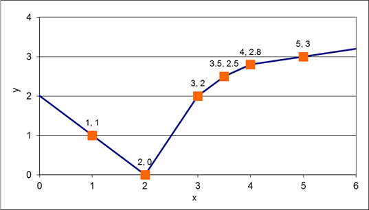
The example shown above demonstrates a PWL function with one input and one output but it can also be extended to cases with multiple inputs and multiple outputs.

MPCCs: Mathematical Programs with Complementarity Constraints

Mathematical Programs with Complementarity Constraints (MPCCs) are formulations that can also be used to model certain classes of discrete events. MPCCs can be more efficient than solving mixed integer formulations of the optimization problems because it avoids the combinatorial difficulties of searching for optimal discrete variables.

• ABS: Absolute Value Operator (MPCC Form)
• MAX: Maximum Operator (MPCC Form)
• MIN: Minimum Operator (MPCC Form)
• Piecewise Linear Function without Object Use (MPCC Form)
• Piecewise Linear Function with PWL Object (MPCC Form)
• Piecewise Linear Function with LOOKUP and PWL Objects (MPCC Form)
• SIGN: Signum Operator (MPCC Form)

Sine Wave Clipping