Model Predictive Control Tutorial
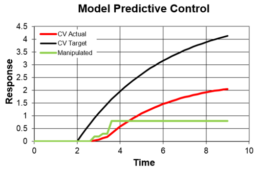
A basic Model Predictive Control (MPC) tutorial demonstrates the capability of a solver to determine a dynamic move plan. In this example, a linear dynamic model is used with the Excel solver to determine a sequence of manipulated variable (MV) adjustments that drive the controlled variable (CV) along a desired reference trajectory.
MATLAB Toolbox for Model Predictive Control
Model Predictive Control (MPC) predicts and optimizes time-varying processes over a future time horizon. This control package accepts linear or nonlinear models. Using large-scale nonlinear programming solvers such as APOPT and IPOPT, it solves data reconciliation, moving horizon estimation, real-time optimization, dynamic simulation, and nonlinear MPC problems.
Download MATLAB Toolbox for Model Predictive Control
Three example files are contained in this directory that implement a controller for Linear Time Invariant (LTI) systems:
- apm1_lti - translate any LTI model into APM format
- apm2_step - perform step tests to ensure model accuracy
- apm3_control - MPC setpoint change to new target values
APMonitor enables the use of empirical, hybrid, and fundamental models directly in control applications. The DBS file parameter IMODE is used to control the simulation mode. This option is set to 6 or 9 for nonlinear control.
 apm.imode = 6 (simultaneous dynamic control)
 apm.imode = 9 (sequential dynamic control)

 % MATLAB example
 apm_option(server,app,'apm.imode',6);

 # Python example
 apm_option(server,app,'apm.imode',9)
Nonlinear control adjusts variables that are declared as Manipulated Variables (MVs) to meet an objective. The MVs are the handles that the optimizer uses to minimize an objective function.
The objective is formulated from Controlled Variables (CVs). The CVs may be controlled to a range, a trajectory, maximized, or minimized. The CVs are an expression of the desired outcome for the controller action.
MPC with Python GEKKO
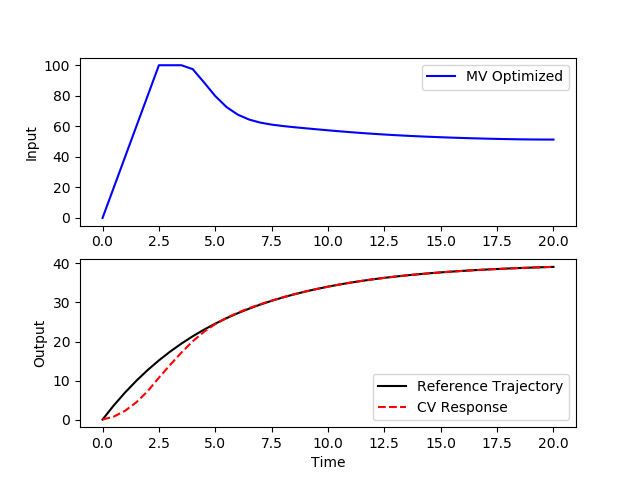
Model Predictive Control (MPC) is also available in the newer Gekko interface with the control option m.options.IMODE=6. A plot of the results can be generated with a plotting package such as Matplotlib. Every time the m.solve() command is called, the solution is time-shifted by one cycle and the MPC calculation repeats with the updated measurements or set points.
import numpy as np
import matplotlib.pyplot as plt
m = GEKKO()
m.time = np.linspace(0,20,41)
# Parameters
mass = 500
b = m.Param(value=50)
K = m.Param(value=0.8)
# Manipulated variable
p = m.MV(value=0, lb=0, ub=100)
p.STATUS = 1 # allow optimizer to change
p.DCOST = 0.1 # smooth out gas pedal movement
p.DMAX = 20 # slow down change of gas pedal
# Controlled Variable
v = m.CV(value=0)
v.STATUS = 1 # add the SP to the objective
m.options.CV_TYPE = 2 # squared error
v.SP = 40 # set point
v.TR_INIT = 1 # set point trajectory
v.TAU = 5 # time constant of trajectory
# Process model
m.Equation(mass*v.dt() == -v*b + K*b*p)
m.options.IMODE = 6 # control
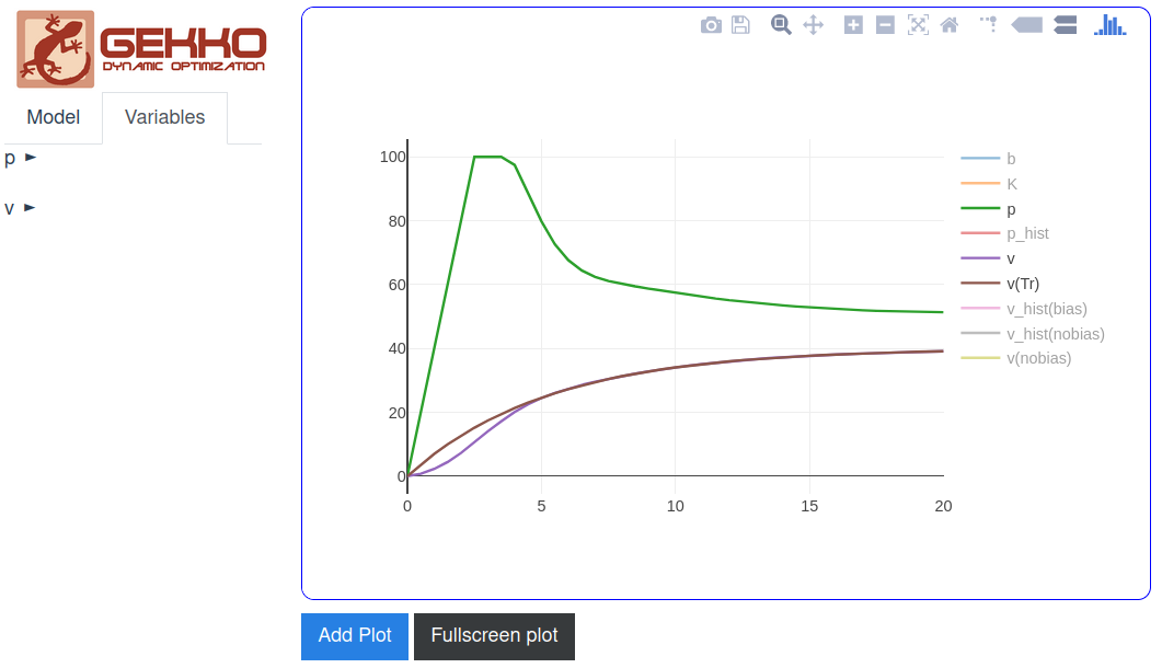
m.solve(disp=False,GUI=True)
# get additional solution information
import json
with open(m.path+'//results.json') as f:
results = json.load(f)
plt.figure()
plt.subplot(2,1,1)
plt.plot(m.time,p.value,'b-',label='MV Optimized')
plt.legend()
plt.ylabel('Input')
plt.subplot(2,1,2)
plt.plot(m.time,results['v1.tr'],'k-',label='Reference Trajectory')
plt.plot(m.time,v.value,'r--',label='CV Response')
plt.ylabel('Output')
plt.xlabel('Time')
plt.legend(loc='best')
plt.show()
The GUI=True option generates a web-interface where FV, MV, SV, and CV types are included with configurable options.
Python Model Predictive Control
Continuous and discrete state space models are used in a Python script for Model Predictive Control. A newer version of the APM Python library is Python Gekko.
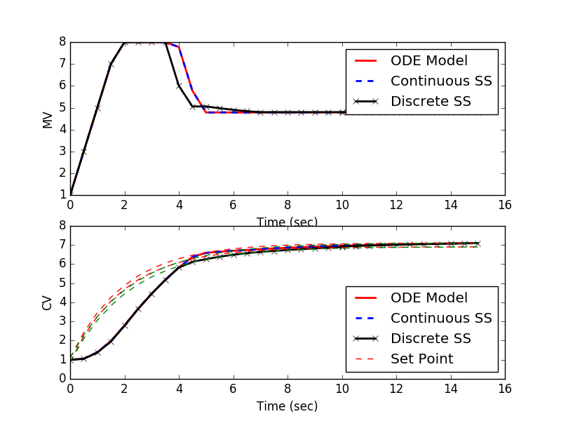
The model1.apm contains a linear first-order differential equation. Other versions are model2.apm (continuous state space) and model3.apm (discrete state space). Each is applied in a model predictive controller to follow a reference trajectory and reach a target value of 7.0.