Simulated annealing is a probabilistic metaheuristic algorithm for approximating the global optimum of a given function. It is a search technique used in optimization for approximating the global optimum of a given function by mimicking the process of annealing in metallurgy. It works by randomly picking a solution from the search space and evaluating its cost, then randomly picking another solution and evaluating its cost and so on until an acceptable solution is found. The process is repeated multiple times with the aim of finding a global optimum solution.
Simulated annealing copies a phenomenon in nature (the annealing of solids) to optimize a complex system. Annealing refers to heating a solid and then cooling it slowly. Complete the following assignment using simulated annealing to arrive at an optimal solution.
Download these files to retrieve the latest versions of the example simulated annealing files in MATLAB and Python. These programs can serve as starting points for designing the homework solutions.
Download Simulated Annealing Example Files

# Import some other libraries that we'll need
# matplotlib and numpy packages must also be installed
import matplotlib
import numpy as np
import matplotlib.pyplot as plt
import random
import math
# define objective function
def f(x):
x1 = x[0]
x2 = x[1]
obj = 0.2 + x1**2 + x2**2 - 0.1*math.cos(6.0*3.1415*x1) - 0.1*math.cos(6.0*3.1415*x2)
return obj
# Start location
x_start = [0.8, -0.5]
# Design variables at mesh points
i1 = np.arange(-1.0, 1.0, 0.01)
i2 = np.arange(-1.0, 1.0, 0.01)
x1m, x2m = np.meshgrid(i1, i2)
fm = np.zeros(x1m.shape)
for i in range(x1m.shape[0]):
for j in range(x1m.shape[1]):
fm[i][j] = 0.2 + x1m[i][j]**2 + x2m[i][j]**2 \
- 0.1*math.cos(6.0*3.1415*x1m[i][j]) \
- 0.1*math.cos(6.0*3.1415*x2m[i][j])
# Create a contour plot
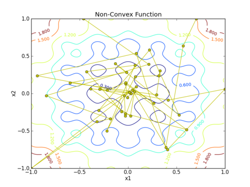
plt.figure()
# Specify contour lines
#lines = range(2,52,2)
# Plot contours
CS = plt.contour(x1m, x2m, fm)#,lines)
# Label contours
plt.clabel(CS, inline=1, fontsize=10)
# Add some text to the plot
plt.title('Non-Convex Function')
plt.xlabel('x1')
plt.ylabel('x2')
##################################################
# Simulated Annealing
##################################################
# Number of cycles
n = 50
# Number of trials per cycle
m = 50
# Number of accepted solutions
na = 0.0
# Probability of accepting worse solution at the start
p1 = 0.7
# Probability of accepting worse solution at the end
p50 = 0.001
# Initial temperature
t1 = -1.0/math.log(p1)
# Final temperature
t50 = -1.0/math.log(p50)
# Fractional reduction every cycle
frac = (t50/t1)**(1.0/(n-1.0))
# Initialize x
x = np.zeros((n+1,2))
x[0] = x_start
xi = np.zeros(2)
xi = x_start
na = na + 1.0
# Current best results so far
xc = np.zeros(2)
xc = x[0]
fc = f(xi)
fs = np.zeros(n+1)
fs[0] = fc
# Current temperature
t = t1
# DeltaE Average
DeltaE_avg = 0.0
for i in range(n):
print('Cycle: ' + str(i) + ' with Temperature: ' + str(t))
for j in range(m):
# Generate new trial points
xi[0] = xc[0] + random.random() - 0.5
xi[1] = xc[1] + random.random() - 0.5
# Clip to upper and lower bounds
xi[0] = max(min(xi[0],1.0),-1.0)
xi[1] = max(min(xi[1],1.0),-1.0)
DeltaE = abs(f(xi)-fc)
if (f(xi)>fc):
# Initialize DeltaE_avg if a worse solution was found
# on the first iteration
if (i==0 and j==0): DeltaE_avg = DeltaE
# objective function is worse
# generate probability of acceptance
p = math.exp(-DeltaE/(DeltaE_avg * t))
# determine whether to accept worse point
if (random.random()<p):
# accept the worse solution
accept = True
else:
# don't accept the worse solution
accept = False
else:
# objective function is lower, automatically accept
accept = True
if (accept==True):
# update currently accepted solution
xc[0] = xi[0]
xc[1] = xi[1]
fc = f(xc)
# increment number of accepted solutions
na = na + 1.0
# update DeltaE_avg
DeltaE_avg = (DeltaE_avg * (na-1.0) + DeltaE) / na
# Record the best x values at the end of every cycle
x[i+1][0] = xc[0]
x[i+1][1] = xc[1]
fs[i+1] = fc
# Lower the temperature for next cycle
t = frac * t
# print solution
print('Best solution: ' + str(xc))
print('Best objective: ' + str(fc))
plt.plot(x[:,0],x[:,1],'y-o')
plt.savefig('contour.png')
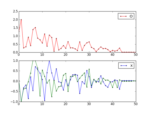
fig = plt.figure()
ax1 = fig.add_subplot(211)
ax1.plot(fs,'r.-')
ax1.legend(['Objective'])
ax2 = fig.add_subplot(212)
ax2.plot(x[:,0],'b.-')
ax2.plot(x[:,1],'g--')
ax2.legend(['x1','x2'])
# Save the figure as a PNG
plt.savefig('iterations.png')
plt.show()
clear;
close all;
%% Generate a contour plot
% Start location
x_start = [0.8, -0.5];
% Design variables at mesh points
i1 = -1.0:0.01:1.0;
i2 = -1.0:0.01:1.0;
[x1m, x2m] = meshgrid(i1, i2);
fm = 0.2 + x1m.^2 + x2m.^2 - 0.1*cos(6.0*pi*x1m) - 0.1*cos(6.0*pi*x2m);
% Contour Plot
fig = figure(1);
[C,h] = contour(x1m,x2m,fm);
clabel(C,h,'Labelspacing',250);
title('Simulated Annealing');
xlabel('x1');
ylabel('x2');
hold on;
%% Simulated Annealing
% Number of cycles
n = 50;
% Number of trials per cycle
m = 50;
% Number of accepted solutions
na = 0.0;
% Probability of accepting worse solution at the start
p1 = 0.7;
% Probability of accepting worse solution at the end
p50 = 0.001;
% Initial temperature
t1 = -1.0/log(p1);
% Final temperature
t50 = -1.0/log(p50);
% Fractional reduction every cycle
frac = (t50/t1)^(1.0/(n-1.0));
% Initialize x
x = zeros(n+1,2);
x(1,:) = x_start;
xi = x_start;
na = na + 1.0;
% Current best results so far
% xc = x(1,:);
fc = f(xi);
fs = zeros(n+1,1);
fs(1,:) = fc;
% Current temperature
t = t1;
% DeltaE Average
DeltaE_avg = 0.0;
for i=1:n
disp(['Cycle: ',num2str(i),' with Temperature: ',num2str(t)])
xc(1) = x(i,1);
xc(2) = x(i,2);
for j=1:m
% Generate new trial points
xi(1) = xc(1) + rand() - 0.5;
xi(2) = xc(2) + rand() - 0.5;
% Clip to upper and lower bounds
xi(1) = max(min(xi(1),1.0),-1.0);
xi(2) = max(min(xi(2),1.0),-1.0);
DeltaE = abs(f(xi)-fc);
if (f(xi)>fc)
% Initialize DeltaE_avg if a worse solution was found
% on the first iteration
if (i==1 && j==1)
DeltaE_avg = DeltaE;
end
% objective function is worse
% generate probability of acceptance
p = exp(-DeltaE/(DeltaE_avg * t));
% % determine whether to accept worse point
if (rand()<p)
% accept the worse solution
accept = true;
else
% don't accept the worse solution
accept = false;
end
else
% objective function is lower, automatically accept
accept = true;
end
% accept
if (accept==true)
% update currently accepted solution
xc(1) = xi(1);
xc(2) = xi(2);
fc = f(xc);
xa(j,1) = xc(1);
xa(j,2) = xc(2);
fa(j) = f(xc);
% increment number of accepted solutions
na = na + 1.0;
% update DeltaE_avg
DeltaE_avg = (DeltaE_avg * (na-1.0) + DeltaE) / na;
else
fa(j) = 0.0;
end
end
% cycle)
fa_Min_Index = find(nonzeros(fa) == min(nonzeros(fa)));
if isempty(fa_Min_Index) == 0
x(i+1,1) = xa(fa_Min_Index,1);
x(i+1,2) = xa(fa_Min_Index,2);
fs(i+1) = fa(fa_Min_Index);
else
x(i+1,1) = x(i,1);
x(i+1,2) = x(i,2);
fs(i+1) = fs(i);
end
% Lower the temperature for next cycle
t = frac * t;
fa = 0.0;
end
% print solution
disp(['Best candidate: ',num2str(xc)])
disp(['Best solution: ',num2str(fc)])
plot(x(:,1),x(:,2),'r-o')
saveas(fig,'contour','png')
fig = figure(2);
subplot(2,1,1)
plot(fs,'r.-')
legend('Objective')
subplot(2,1,2)
hold on
plot(x(:,1),'b.-')
plot(x(:,2),'g.-')
legend('x_1','x_2')
% Save the figure as a PNG
saveas(fig,'iterations','png')
Save as f.m
x1 = x(1);
x2 = x(2);
obj = 0.2 + x1^2 + x2^2 - 0.1*cos(6.0*pi*x1) - 0.1*cos(6.0*pi*x2);
end
 This assignment can be completed in groups of two. Additional guidelines on individual, collaborative, and group assignments are provided under the Expectations link.