Design Optimization

m.Minimize(((y-z)/z)**2)

(:title Nonlinear and Multivariate Regression:)

Objective: Perform nonlinear and multivariate regression on energy data to predict oil price.

Predictors are data features that are inputs to calculate a predicted output. In machine learning the data inputs are called features and the measured outputs are called labels. Regression is the method of adjusting parameters in a model to minimize the difference between the predicted output and the measured output. The objective of this problem is to predict the price of oil (OIL) from indicator features that include West Texas Intermediate (WTI) price, Henry Hub gas price (HH), and the Mont Belvieu (MB) propane spot price. Data is available for OIL, WTI, HH, and MB from the years 2000 to 2016 at the following link.

There is additional information about regression in the Data Science Online Course.

This particular nonlinear equation can be transformed to a linear equation with a log transformation as

$$\log(OIL)=\log(A)+B\log(WTI)+C\log(HH)+D\log(MB)$$

or kept in the original nonlinear form. Adjust the unknown parameters (A, B, C, D) to minimize a sum of squared errors of the normalized difference between the measured and predicted value. Normalize the difference by the measured value before the it is squared.

This particular nonlinear equation can be transformed to a linear equation with a log transformation as `\log(OIL)=\log(A)+B\log(WTI)+C\log(HH)+D\log(MB)` or kept in the original nonlinear form. Adjust the unknown parameters (A, B, C, D) to minimize a sum of squared errors of the normalized difference between the measured and predicted value. Normalize the difference by the measured value before the it is squared.

This particular nonlinear equation can be transformed to a linear equation with a log transformation as `\log(OIL)=\log(A)+B\,\log(WTI)+C\,log(HH)+D\,log(MB)` or kept in the original nonlinear form. Adjust the unknown parameters (A, B, C, D) to minimize a sum of squared errors of the normalized difference between the measured and predicted value. Normalize the difference by the measured value before the it is squared.

(:html:) <iframe width="560" height="315" src="https://www.youtube.com/embed/BSwm2ZSstEY" frameborder="0" allow="autoplay; encrypted-media" allowfullscreen></iframe> (:htmlend:)

(:title Nonlinear Regression with Energy Prices:)

Python (GEKKO) Solution

1. use 'pip install gekko' to get package

Python (SciPy) Solution

1. Energy price non-linear regression
2. solve for oil sales price (outcome)
3. using 3 predictors of WTI Oil Price,
4. Henry Hub Price and MB Propane Spot Price

import numpy as np from scipy.optimize import minimize import pandas as pd import numpy as np import matplotlib.pyplot as plt

1. data file from URL address

data = 'https://apmonitor.com/me575/uploads/Main/oil_data.txt' df = pd.read_csv(data)

xm1 = np.array(df["WTI_PRICE"]) # WTI Oil Price xm2 = np.array(df["HH_PRICE"]) # Henry Hub Gas Price xm3 = np.array(df["NGL_PRICE"]) # MB Propane Spot Price ym = np.array(df["BEST_PRICE"]) # oil sales price received (outcome)

1. calculate y

def calc_y(x):

    a = x[0]
    b = x[1]
    c = x[2]
    d = x[3]
    #y = a * xm1 + b  # linear regression
    y = a * ( xm1 ** b ) * ( xm2 ** c ) * ( xm3 ** d )
    return y

1. define objective

def objective(x):

    # calculate y
    y = calc_y(x)
    # calculate objective
    obj = 0.0
    for i in range(len(ym)):
        obj = obj + ((y[i]-ym[i])/ym[i])**2    
    # return result
    return obj

1. initial guesses

x0 = np.zeros(4) x0[0] = 0.0 # a x0[1] = 0.0 # b x0[2] = 0.0 # c x0[3] = 0.0 # d

1. show initial objective

print('Initial Objective: ' + str(objective(x0)))

1. optimize
2. bounds on variables

my_bnds = (-100.0, 100.0) bnds = (my_bnds, my_bnds, my_bnds, my_bnds) solution = minimize(objective, x0, method='SLSQP', bounds=bnds) x = solution.x y = calc_y(x)

1. show final objective

cObjective = 'Final Objective: ' + str(objective(x)) print(cObjective)

1. print solution

print('Solution')

cA = 'A = ' + str(x[0]) print(cA) cB = 'B = ' + str(x[1]) print(cB) cC = 'C = ' + str(x[2]) print(cC) cD = 'D = ' + str(x[3]) print(cD)

cFormula = "Formula is : " + "\n" + "A * WTI^B * HH^C * PROPANE^D" cLegend = cFormula + "\n" + cA + "\n" + cB + "\n" + cC + "\n" + cD + "\n" + cObjective

1. ym measured outcome
2. y predicted outcome

from scipy import stats slope, intercept, r_value, p_value, std_err = stats.linregress(ym,y) r2 = r_value**2 cR2 = "R^2 correlation = " + str(r_value**2) print(cR2)

1. plot solution

plt.figure(1) plt.title('Actual (YM) versus Predicted (Y) Outcomes For Non-Linear Regression') plt.plot(ym,y,'o') plt.xlabel('Measured Outcome (YM)') plt.ylabel('Predicted Outcome (Y)') plt.legend([cLegend]) plt.grid(True) plt.show()

(:toggle hide scipy button show="Show Python (SciPy) Code":) (:div id=scipy:)

Adjust the unknown parameters (A, B, C, D) to minimize a sum of squared errors of the normalized difference between the measured and predicted value. Normalize the difference by the measured value before the it is squared.

$$\min_{A,B,C,D} \sum_{i=1}^n \left( \frac{OIL_{pred,i}-OIL_{meas,i}}{OIL_{meas,i}} \right)^2$$

where n is the number of data points, i is an index for the current measured value, pred is the predicted value, and meas is the measured value. Report the parameter values, the R² value of fit, and display a plot of the results.

1. Energy price non-linear regression
2. solve for oil sales price (outcome)
3. using 3 predictors of WTI Oil Price,
4. Henry Hub Price and MB Propane Spot Price

import numpy as np from gekko import GEKKO import pandas as pd import numpy as np import matplotlib.pyplot as plt

1. data file from URL address

data = 'https://apmonitor.com/me575/uploads/Main/oil_data.txt' df = pd.read_csv(data)

xm1 = np.array(df["WTI_PRICE"]) # WTI Oil Price xm2 = np.array(df["HH_PRICE"]) # Henry Hub Gas Price xm3 = np.array(df["NGL_PRICE"]) # MB Propane Spot Price ym = np.array(df["BEST_PRICE"]) # oil sales price

1. GEKKO model

m = GEKKO() a = m.FV(lb=-100.0,ub=100.0) b = m.FV(lb=-100.0,ub=100.0) c = m.FV(lb=-100.0,ub=100.0) d = m.FV(lb=-100.0,ub=100.0) x1 = m.Param(value=xm1) x2 = m.Param(value=xm2) x3 = m.Param(value=xm3) z = m.Param(value=ym) y = m.Var() m.Equation(y==a*(x1**b)*(x2**c)*(x3**d)) m.Obj(((y-z)/z)**2)

1. Options

a.STATUS = 1 b.STATUS = 1 c.STATUS = 1 d.STATUS = 1 m.options.IMODE = 2 m.options.SOLVER = 1

1. Solve

m.solve()

print('a: ', a.value[0]) print('b: ', b.value[0]) print('c: ', c.value[0]) print('d: ', d.value[0])

cFormula = "Formula is : " + "\n" + r"$A * WTI^B * HH^C * PROPANE^D$"

from scipy import stats slope, intercept, r_value, p_value, std_err = stats.linregress(ym,y)

r2 = r_value**2 cR2 = "R^2 correlation = " + str(r_value**2) print(cR2)

1. plot solution

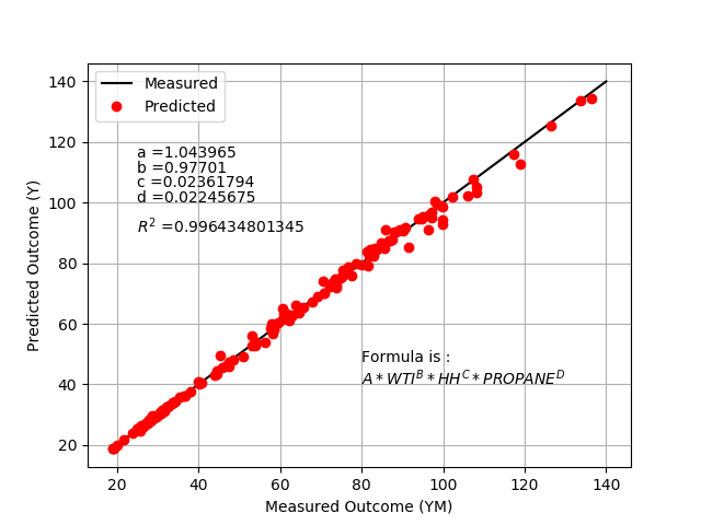
plt.figure(1) plt.plot([20,140],[20,140],'k-',label='Measured') plt.plot(ym,y,'ro',label='Predicted') plt.xlabel('Measured Outcome (YM)') plt.ylabel('Predicted Outcome (Y)') plt.legend(loc='best') plt.text(25,115,'a =' + str(a.value[0])) plt.text(25,110,'b =' + str(b.value[0])) plt.text(25,105,'c =' + str(c.value[0])) plt.text(25,100,'d =' + str(d.value[0])) plt.text(25,90,r'$R^2$ =' + str(r_value**2)) plt.text(80,40,cFormula) plt.grid(True) plt.show()

$$OIL = A \, \left(WTI^B\right) \, \left(HH^C\right) \, \left(MB^D\right)$$

(:title Nonlinear Regression with Energy Price Example:) (:keywords Nonlinear Regression, Factors, Multivariate, Optimization, Constraint, Nonlinear Programming:) (:description Perform nonlinear regression on energy data to predict oil price.:)

Predict the price of oil (OIL) from indicators such as the West Texas Intermediate (WTI) price, Henry Hub gas price (HH), and the Mont Belvieu (MB) propane spot price. Data is available for OIL, WTI, HH, and MB from the years 2000 to 2016 at the following link.

Oil Data (oil_data.csv) Δ

Use the following nonlinear correlation with unknown parameters A, B, C, and D.

$$OIL = A \, WTI^B \, HH^C \, MB^D$$

Adjust the unknown parameters (A, B, C, D) to minimize a sum of squared errors of the normalized difference between the measured and predicted value. Normalize the difference by the measured value before the it is squared. Report the parameter values, the R² value of fit, and display a plot of the results.

(:toggle hide gekko button show="Show Python (GEKKO) Code":) (:div id=gekko:) (:source lang=python:)

(:sourceend:) (:divend:)

(:toggle hide gekko button show="Show Python (SciPy) Code":) (:div id=gekko:) (:source lang=python:)

(:sourceend:) (:divend:)

Thanks to Fulton Loebel for submitting this example problem to the APMonitor Discussion Forum.

(:html:)

 <div id="disqus_thread"></div>
    <script type="text/javascript">
        /* * * CONFIGURATION VARIABLES: EDIT BEFORE PASTING INTO YOUR WEBPAGE * * */
        var disqus_shortname = 'apmonitor'; // required: replace example with your forum shortname

        /* * * DON'T EDIT BELOW THIS LINE * * */
        (function() {
            var dsq = document.createElement('script'); dsq.type = 'text/javascript'; dsq.async = true;
            dsq.src = 'https://' + disqus_shortname + '.disqus.com/embed.js';
            (document.getElementsByTagName('head')[0] || document.getElementsByTagName('body')[0]).appendChild(dsq);
        })();
    </script>
    <noscript>Please enable JavaScript to view the <a href="https://disqus.com/?ref_noscript">comments powered by Disqus.</a></noscript>
    <a href="https://disqus.com" class="dsq-brlink">comments powered by <span class="logo-disqus">Disqus</span></a>

(:htmlend:)