Linear programming (LP) is a mathematical optimization technique used to solve problems with a linear objective function and linear constraints. Linear Programming maximizes or minimizes a linear objective function of several variables subject to constraints that are also linear in the same variables.
See Optimization with Python for examples of:
- 1️⃣ Linear Programming (LP)
- 2️⃣ Quadratic Programming (QP)
- 3️⃣ Nonlinear Programming (NLP)
- 4️⃣ Mixed Integer Linear Programming (MILP)
- 5️⃣ Mixed Integer Nonlinear Programming (MINLP)
Linear programming is widely used in engineering decision-making to optimize resource allocation, such as minimize costs, maximize profits, or maximize output, subject to a set of constraints. For example, a refinery might use linear programming to determine the optimal crude oils to purchase to maximize profit from their specific equipment that is subject to processing constraints and can make a certain amount of each refined product. Linear programming can also be used to solve complex logistical problems, such as a schedule production runs, determine optimal transportation routes, and minimize inventory costs.
An advantage of linear programming over nonlinear programming is the ability to handle a large number of variables and constraints, model complex situations, and provide an explainable, quantitative basis for decision-making. By using linear programming, engineers can make more informed decisions, reduce costs, and increase efficiency.
Refinery Example LP Problem
A refinery must produce 100 gallons of gasoline and 160 gallons of diesel to meet customer demands. The refinery would like to minimize the cost of crude and two crude options exist. The less expensive crude costs $80 USD per barrel while a more expensive crude costs $95 USD per barrel. Each barrel of the less expensive crude produces 10 gallons of gasoline and 20 gallons of diesel. Each barrel of the more expensive crude produces 15 gallons of both gasoline and diesel. Find the number of barrels of each crude that will minimize the refinery cost while satisfying the customer demands.
Refinery Optimization with Linear Programming
- Solve Refinery Optimization Problem with Continuous Variables
Refinery Optimization with Mixed Integer Linear Programming
- Solve Refinery Optimization Problem with Integer Variables
Soft Drink Production Problem (Example 2)
A simple production planning problem is given by the use of two ingredients A and B that produce products 1 and 2. The available supply of A is 30 units and B is 44 units. For production it requires:
- 3 units of A and 8 units of B to produce Product 1
- 6 units of A and 4 units of B to produce Product 2
There are at most 5 units of Product 1 and 4 units of Product 2. Product 1 can be sold for 100 and Product 2 can be sold for 125. The objective is to maximize the profit for this production problem.
Python Solution
m = GEKKO()
x1 = m.Var(lb=0,ub=5)
x2 = m.Var(lb=0,ub=4)
profit = m.Var()
m.Maximize(profit) # maximize
m.Equation(profit==100*x1 + 125*x2)
m.Equation(3*x1+6*x2<=30)
m.Equation(8*x1+4*x2<=44)
m.solve()
print ('')
print ('--- Results of the Optimization Problem ---')
print ('Product 1 (x1): ' + str(x1.value))
print ('Product 2 (x2): ' + str(x2.value))
print ('Profit: ' + str(profit.value))
See additional solution options for solving Linear Programming with Python.
Contour Plot
A contour plot can be used to explore the optimal solution. In this case, the black lines indicate the upper and lower bounds on the production of 1 and 2. In this case, the production of 1 must be greater than 0 but less than 5. The production of 2 must be greater than 0 but less than 4.
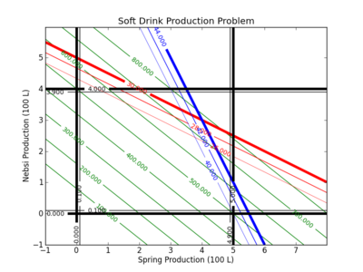
Soft Drink Production Problem
Solve the Production Problem Online
Modified Production Problem
Solve the Modified Production Problem Online
Solution and Contour Plots with Python
Below are the source files for generating the contour plots in GEKKO Python and APM Python.
m = GEKKO()
x1 = m.Var(lb=0,ub=5)
x2 = m.Var(lb=0,ub=4)
profit = m.Var()
m.Maximize(profit)
m.Equation(profit==100*x1 + 125*x2)
m.Equation(3*x1+6*x2<=30)
m.Equation(8*x1+4*x2<=44)
m.solve()
print ('')
print ('--- Results of the Optimization Problem ---')
print ('Product 1 (x1): ' + str(x1.value))
print ('Product 2 (x2): ' + str(x2.value))
print ('Profit: ' + str(profit.value))
## Generate a contour plot
# Import some other libraries that we'll need
# matplotlib and numpy packages must also be installed
import matplotlib
import numpy as np
import matplotlib.pyplot as plt
# Design variables at mesh points
x = np.arange(-1.0, 8.0, 0.02)
y = np.arange(-1.0, 6.0, 0.02)
x1, x2 = np.meshgrid(x,y)
# Equations and Constraints
profit = 100.0 * x1 + 125.0 * x2
A_usage = 3.0 * x1 + 6.0 * x2
B_usage = 8.0 * x1 + 4.0 * x2
# Create a contour plot
plt.figure()
# Weight contours
lines = np.linspace(100.0,800.0,8)
CS = plt.contour(x1,x2,profit,lines,colors='g')
plt.clabel(CS, inline=1, fontsize=10)
# A usage < 30
CS = plt.contour(x1,x2,A_usage,[26.0, 28.0, 30.0],colors='r',linewidths=[0.5,1.0,4.0])
plt.clabel(CS, inline=1, fontsize=10)
# B usage < 44
CS = plt.contour(x1, x2,B_usage,[40.0,42.0,44.0],colors='b',linewidths=[0.5,1.0,4.0])
plt.clabel(CS, inline=1, fontsize=10)
# Container for 0 <= Product 1 <= 500 L
CS = plt.contour(x1, x2,x1 ,[0.0, 0.1, 4.9, 5.0],colors='k',linewidths=[4.0,1.0,1.0,4.0])
plt.clabel(CS, inline=1, fontsize=10)
# Container for 0 <= Product 2 <= 400 L
CS = plt.contour(x1, x2,x2 ,[0.0, 0.1, 3.9, 4.0],colors='k',linewidths=[4.0,1.0,1.0,4.0])
plt.clabel(CS, inline=1, fontsize=10)
# Add some labels
plt.title('Soft Drink Production Problem')
plt.xlabel('Product 1 (100 L)')
plt.ylabel('Product 2 (100 L)')
# Save the figure as a PNG
plt.savefig('contour.png')
# Show the plots
plt.show()