Dynamic Optimization

        plt.plot(tm[0:i],Q1s[0:i],'r-',lw=3,label=r'$Q_1$')
        plt.plot(tm[0:i],Q2s[0:i],'b:',lw=3,label=r'$Q_2$')

                 label=r'$T_1$ target',lw=3)

                 label=None,lw=3)

                 label=r'$T_1$ predicted',lw=3)

                 label=r'$T_2$ target',lw=3)

                 label=None,lw=3)

                 label=r'$T_2$ predict',lw=3)

                 label='Current Time',lw=1)

                 label=r'$Q_1$ history',lw=2)

                 label=r'$Q_1$ plan',lw=3)

                 label=r'$Q_2$ history',lw=2)

                 label=r'$Q_2$ plan',lw=3)

                 label=r'$T_1$ target',lw=3)

                 label=None,lw=3)

                 label=r'$T_1$ predicted',lw=3)

                 label=r'$T_2$ target',lw=3)

                 label=None,lw=3)

                 label=r'$T_2$ predict',lw=3)

                 label='Current Time',lw=1)

                 label=r'$Q_1$ history',lw=2)

                 label=r'$Q_1$ plan',lw=3)

                 label=r'$Q_2$ history',lw=2)

                 label=r'$Q_2$ plan',lw=3)

See SISO Model Identification for information on creating a single heater, single temperature control model.

TCLab F: SISO Control Jupyter Notebook

See MIMO Model Identification for additional help on creating and step testing a MIMO (Multiple Input, Multiple Output) Auto-regressive exogenous (ARX) input model.

Virtual TCLab on Google Colab

TC1 = m.CV(value=TC1_ss.value)

m = GEKKO()

y = m.Array(m.CV,2) u = m.Array(m.MV,2) m.arx(p,y,u)

na = 2 # output coefficients nb = 2 # input coefficients

yp,p,K = m.sysid(t,u,y,na,nb,objf=10000,scale=False,diaglevel=1)

m.time=np.linspace(0,120,61)

Q1.DMAX = 50.0

Q2.DMAX = 50.0

TC1.TAU = 20 # response speed (time constant) TC1.TR_INIT = 2 # reference trajectory

TC2.TAU = 20 # response speed (time constant) TC2.TR_INIT = 2 # dead-band

na = 1 # output coefficients nb = 1 # input coefficients

yp,p,K = m.sysid(t,u,y,na,nb,scale=False,objf=100)

plt.show()

import numpy as np import time import matplotlib.pyplot as plt import pandas as pd import json

1. get gekko package with:
2. pip install gekko

from gekko import GEKKO

1. get tclab package with:
2. pip install tclab

from tclab import TCLab

1. Connect to Arduino

a = TCLab()

1. Make an MP4 animation?

make_mp4 = False if make_mp4:

    import imageio  # required to make animation
    import os
    try:
        os.mkdir('./figures')
    except:
        pass

1. Final time

tf = 10 # min

1. number of data points (every 2 seconds)

n = tf * 30 + 1

1. Percent Heater (0-100%)

Q1s = np.zeros(n) Q2s = np.zeros(n)

1. Temperatures (degC)

T1m = a.T1 * np.ones(n) T2m = a.T2 * np.ones(n)

1. Temperature setpoints

T1sp = T1m[0] * np.ones(n) T2sp = T2m[0] * np.ones(n)

1. Heater set point steps about every 150 sec

T1sp[3:] = 50.0 T2sp[40:] = 35.0 T1sp[80:] = 30.0 T2sp[120:] = 50.0 T1sp[160:] = 45.0 T2sp[200:] = 35.0 T1sp[240:] = 60.0

1. Initialize Model

2. load data (20 min, dt=2 sec) and parse into columns

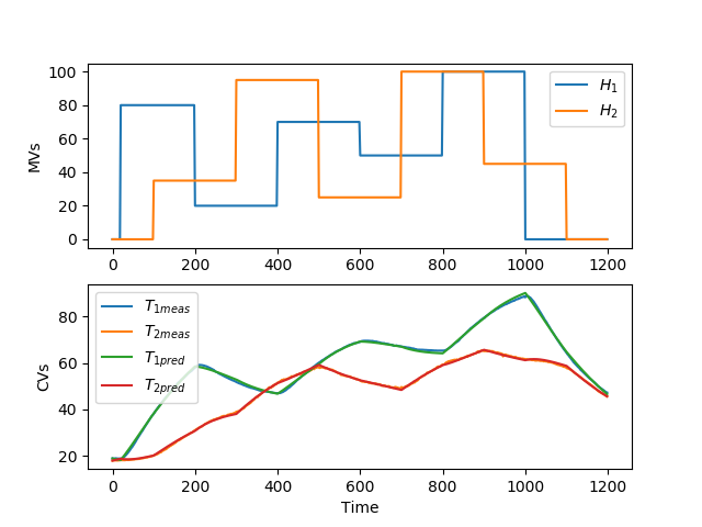
url = 'http://apmonitor.com/do/uploads/Main/tclab_2sec.txt' data = pd.read_csv(url) t = data['Time'] u = data'H1','H2'? y = data'T1','T2'?

1. generate time-series model

m = GEKKO(remote=False)

1. system identification

na = 2 # output coefficients nb = 2 # input coefficients print('Identify model') yp,p,K = m.sysid(t,u,y,na,nb)

1. plot sysid results

plt.figure() plt.subplot(2,1,1) plt.plot(t,u) plt.legend([r'$H_1$',r'$H_2$']) plt.ylabel('MVs') plt.subplot(2,1,2) plt.plot(t,y) plt.plot(t,yp) plt.legend([r'$T_{1meas}$',r'$T_{2meas}$', r'$T_{1pred}$',r'$T_{2pred}$']) plt.ylabel('CVs') plt.xlabel('Time') plt.savefig('sysid.png')

1. create control ARX model

y,u = m.arx(p)

1. rename CVs

TC1 = y[0] TC2 = y[1]

1. rename MVs

Q1 = u[0] Q2 = u[1]

1. steady state initialization

m.options.IMODE = 1 m.solve(disp=False)

1. set up MPC

m.options.IMODE = 6 # MPC m.options.CV_TYPE = 1 # Objective type m.options.NODES = 2 # Collocation nodes m.options.SOLVER = 3 # IPOPT m.time=np.linspace(0,60,61)

1. Manipulated variables

Q1.STATUS = 1 # manipulated Q1.FSTATUS = 0 # not measured Q1.DMAX = 20.0 Q1.DCOST = 0.1 Q1.UPPER = 100.0 Q1.LOWER = 0.0

Q2.STATUS = 1 # manipulated Q2.FSTATUS = 0 # not measured Q2.DMAX = 30.0 Q2.DCOST = 0.1 Q2.UPPER = 100.0 Q2.LOWER = 0.0

1. Controlled variables

TC1.STATUS = 1 # drive to set point TC1.FSTATUS = 1 # receive measurement TC1.TAU = 40 # response speed (time constant) TC1.TR_INIT = 1 # reference trajectory TC1.TR_OPEN = 0

TC2.STATUS = 1 # drive to set point TC2.FSTATUS = 1 # receive measurement TC2.TAU = 0 # response speed (time constant) TC2.TR_INIT = 0 # dead-band TC2.TR_OPEN = 1

1. Create plot

plt.figure(figsize=(10,7)) plt.ion() plt.show()

1. Main Loop

start_time = time.time() prev_time = start_time tm = np.zeros(n)

try:

    for i in range(1,n-1):
        # Sleep time
        sleep_max = 2.0
        sleep = sleep_max - (time.time() - prev_time)
        if sleep>=0.01:
            time.sleep(sleep-0.01)
        else:
            time.sleep(0.01)

        # Record time and change in time
        t = time.time()
        dt = t - prev_time
        prev_time = t
        tm[i] = t - start_time

        # Read temperatures in Celsius 
        T1m[i] = a.T1
        T2m[i] = a.T2

        # Insert measurements
        TC1.MEAS = T1m[i]
        TC2.MEAS = T2m[i]

        # Adjust setpoints
        db1 = 1.0 # dead-band
        TC1.SPHI = T1sp[i] + db1
        TC1.SPLO = T1sp[i] - db1

        db2 = 0.2
        TC2.SPHI = T2sp[i] + db2
        TC2.SPLO = T2sp[i] - db2

        # Adjust heaters with MPC
        m.solve() 

        if m.options.APPSTATUS == 1:
            # Retrieve new values
            Q1s[i+1]  = Q1.NEWVAL
            Q2s[i+1]  = Q2.NEWVAL
            # get additional solution information
            with open(m.path+'//results.json') as f:
                results = json.load(f)
        else:
            # Solution failed
            Q1s[i+1]  = 0.0
            Q2s[i+1]  = 0.0

        # Write new heater values (0-100)
        a.Q1(Q1s[i])
        a.Q2(Q2s[i])

        # Plot
        plt.clf()
        ax=plt.subplot(3,1,1)
        ax.grid()
        plt.plot(tm[0:i+1],T1sp[0:i+1]+db1,'k-',                 label=r'$T_1$ target',linewidth=3)
        plt.plot(tm[0:i+1],T1sp[0:i+1]-db1,'k-',                 label=None,linewidth=3)
        plt.plot(tm[0:i+1],T1m[0:i+1],'r.',label=r'$T_1$ measured')
        plt.plot(tm[i]+m.time,results['v1.bcv'],'r-',                 label=r'$T_1$ predicted',linewidth=3)
        plt.plot(tm[i]+m.time,results['v1.tr_hi'],'k--',                 label=r'$T_1$ trajectory')
        plt.plot(tm[i]+m.time,results['v1.tr_lo'],'k--')
        plt.ylabel('Temperature (degC)')
        plt.legend(loc=2)
        ax=plt.subplot(3,1,2)
        ax.grid()        
        plt.plot(tm[0:i+1],T2sp[0:i+1]+db2,'k-',                 label=r'$T_2$ target',linewidth=3)
        plt.plot(tm[0:i+1],T2sp[0:i+1]-db2,'k-',                 label=None,linewidth=3)
        plt.plot(tm[0:i+1],T2m[0:i+1],'b.',label=r'$T_2$ measured')
        plt.plot(tm[i]+m.time,results['v2.bcv'],'b-',                 label=r'$T_2$ predict',linewidth=3)
        plt.plot(tm[i]+m.time,results['v2.tr_hi'],'k--',                 label=r'$T_2$ range')
        plt.plot(tm[i]+m.time,results['v2.tr_lo'],'k--')
        plt.ylabel('Temperature (degC)')
        plt.legend(loc=2)
        ax=plt.subplot(3,1,3)
        ax.grid()
        plt.plot([tm[i],tm[i]],[0,100],'k-',                 label='Current Time',linewidth=1)
        plt.plot(tm[0:i+1],Q1s[0:i+1],'r.-',                 label=r'$Q_1$ history',linewidth=2)
        plt.plot(tm[i]+m.time,Q1.value,'r-',                 label=r'$Q_1$ plan',linewidth=3)
        plt.plot(tm[0:i+1],Q2s[0:i+1],'b.-',                 label=r'$Q_2$ history',linewidth=2)
        plt.plot(tm[i]+m.time,Q2.value,'b-',
                 label=r'$Q_2$ plan',linewidth=3)
        plt.plot(tm[i]+m.time[1],Q1.value[1],color='red',                 marker='.',markersize=15)
        plt.plot(tm[i]+m.time[1],Q2.value[1],color='blue',                 marker='X',markersize=8)
        plt.ylabel('Heaters')
        plt.xlabel('Time (sec)')
        plt.legend(loc=2)
        plt.draw()
        plt.pause(0.05)
        if make_mp4:
            filename='./figures/plot_str(i+10000).png'
            plt.savefig(filename)

    # Turn off heaters and close connection
    a.Q1(0)
    a.Q2(0)
    a.close()
    # Save figure
    plt.savefig('tclab_mpc.png')

    # generate mp4 from png figures in batches of 350
    if make_mp4:
        images = []
        iset = 0
        for i in range(1,n-1):
            filename='./figures/plot_str(i+10000).png'
            images.append(imageio.imread(filename))
            if ((i+1)%350)==0:
                imageio.mimsave('results_str(iset).mp4', images)
                iset += 1
                images = []
        if images!=[]:
            imageio.mimsave('results_str(iset).mp4', images)

1. Allow user to end loop with Ctrl-C

except KeyboardInterrupt:

    # Turn off heaters and close connection
    a.Q1(0)
    a.Q2(0)
    a.close()
    print('Shutting down')
    plt.savefig('tclab_mpc.png')

1. Make sure serial connection still closes when there's an error

except:

    # Disconnect from Arduino
    a.Q1(0)
    a.Q2(0)
    a.close()
    print('Error: Shutting down')
    plt.savefig('tclab_mpc.png')
    raise

    fid.close()

plt.savefig('tclab_dyn_2sec.png')

See MIMO Model Identification for additional help on creating and step testing an Auto-regressive exogenous (ARX) model.

Attach:tclab_arx_mpc.mp4

(:html:) <video width="550" controls autoplay loop>

  <source src="/do/uploads/Main/tclab_arx_mpc.mp4" type="video/mp4">
  Your browser does not support the video tag.

</video> (:htmlend:)

TCLab Step Test Data for ARX Fit (20 min with `\Delta t` = 2 sec)

Python GEKKO System ID with ARX Model

Attach:tclab_arx_mpc.mp4

  <source src="/do/uploads/Main/tclab_arx_mpc.mp4" type="video/mp4">

Attach:tclab_arx_step_test.

    fid.write(str(2*i)+',str(Q1d[i]),str(Q2d[i]),' \

Python GEKKO 1st Order Model

Python GEKKO 2nd Order Model

(:sourceend:) (:divend:)

Python GEKKO 2nd Order Model

(:html:) <video width="550" controls autoplay loop>

  <source src="/do/uploads/Main/tclab_linear_mpc.mp4" type="video/mp4">
  Your browser does not support the video tag.

</video> (:htmlend:)

(:toggle hide gekko_labF3 button show="Lab F: Python TCLab Generate Data for ARX":) (:div id=gekko_labF3:) (:source lang=python:) import numpy as np import pandas as pd import tclab import time import matplotlib.pyplot as plt

1. generate step test data on Arduino

filename = 'tclab_2sec.csv'

1. heater steps

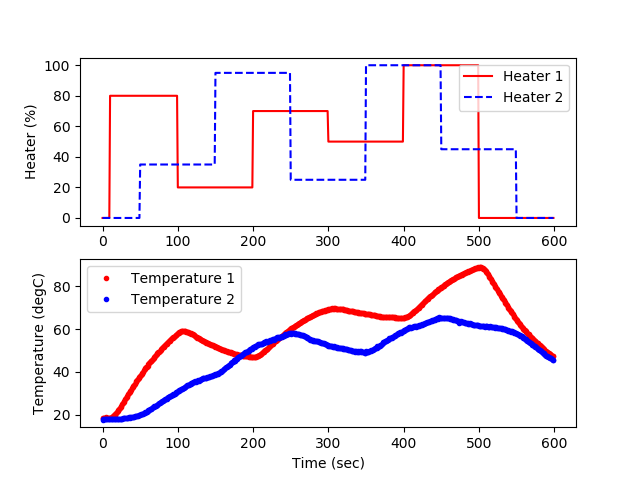
Q1d = np.zeros(601) Q1d[10:100] = 80 Q1d[100:200] = 20 Q1d[200:300] = 70 Q1d[300:400] = 50 Q1d[400:500] = 100 Q1d[500:] = 0

Q2d = np.zeros(601) Q2d[50:150] = 35 Q2d[150:250] = 95 Q2d[250:350] = 25 Q2d[350:450] = 100 Q2d[450:550] = 45 Q2d[550:] = 0

1. Connect to Arduino

a = tclab.TCLab() fid = open(filename,'w') fid.write('Time,H1,H2,T1,T2\n') fid.close()

1. run step test (20 min)

for i in range(601):

    # set heater values
    a.Q1(Q1d[i])
    a.Q2(Q2d[i])
    print('Time: ' + str(2*i) +           ' H1: ' + str(Q1d[i]) +           ' H2: ' + str(Q2d[i]) +           ' T1: ' + str(a.T1)   +           ' T2: ' + str(a.T2))
    # wait 2 seconds
    time.sleep(2)
    fid = open(filename,'a')
    fid.write(str(i)+',str(Q1d[i]),str(Q2d[i]),'               +str(a.T1)+',str(a.T2)\n')

1. close connection to Arduino

a.close()

1. read data file

data = pd.read_csv(filename)

1. plot measurements

plt.figure() plt.subplot(2,1,1) plt.plot(data['Time'],data['H1'],'r-',label='Heater 1') plt.plot(data['Time'],data['H2'],'b--',label='Heater 2') plt.ylabel('Heater (%)') plt.legend(loc='best') plt.subplot(2,1,2) plt.plot(data['Time'],data['T1'],'r.',label='Temperature 1') plt.plot(data['Time'],data['T2'],'b.',label='Temperature 2') plt.ylabel('Temperature (degC)') plt.legend(loc='best') plt.xlabel('Time (sec)') plt.savefig('tclab_dyn_meas2.png')

plt.show() (:sourceend:) (:divend:)

TCLab Step Test Data for ARX Fit (`\Delta t` = 2 sec

(:toggle hide gekko_labF4 button show="Lab F: Python TCLab MIMO MPC with ARX Model":) (:div id=gekko_labF4:) Note: Switch to make_mp4 = True to make an MP4 movie animation. This requires imageio and ffmpeg (install available through Python). It creates a folder named figures in your run directory. You can delete this folder after the run is complete.

(:source lang=python:)

Note: Switch to make_mp4 = True to make an MP4 movie animation. This requires imageio and ffmpeg (install available through Python). It creates a folder named figures in your run directory. You can delete this folder after the run is complete.

        # Adjust heaters with MPC

m.options.CV_TYPE = 1 # Objective type

1. Initialize Model

1. Manipulated variables

Q1.FSTATUS = 0 # not measured

Q2.FSTATUS = 0 # not measured

1. Controlled variables

TC1.STATUS = 1 # drive to set point

TC2.STATUS = 1 # drive to set point

m.options.IMODE = 6 # MPC

1. Initialize Model

m = GEKKO(name='tclab-mpc',remote=False)

1. with a local server
2. m = GEKKO(name='tclab-mpc',server='http://127.0.0.1',remote=True)

Attach:tclab_linear_mpc.mp4

(:html:) <video width="550" controls autoplay loop>

  <source src="/do/uploads/Main/tclab_linear_mpc.mp4" type="video/mp4">
  Your browser does not support the video tag.

</video> (:htmlend:)

import json

1. Make an MP4 animation?

make_mp4 = False if make_mp4:

    import imageio  # required to make animation
    import os
    try:
        os.mkdir('./figures')
    except:
        pass

1. m = GEKKO(name='tclab-mpc',remote=False)

m = GEKKO(name='tclab-mpc',server='http://127.0.0.1',remote=True)

Q1 = m.MV(value=0,name='q1')

Q2 = m.MV(value=0,name='q2')

TC1 = m.CV(value=T1m[0],name='tc1')

TC1.TAU = 40 # response speed (time constant) TC1.TR_INIT = 1 # reference trajectory TC1.TR_OPEN = 0

TC2 = m.CV(value=T2m[0],name='tc2')

TC2.TAU = 0 # response speed (time constant) TC2.TR_INIT = 0 # dead-band TC2.TR_OPEN = 1

    for i in range(1,n-1):

        db1 = 1.0 # dead-band
        TC1.SPHI = T1sp[i] + db1
        TC1.SPLO = T1sp[i] - db1

        db2 = 0.2
        TC2.SPHI = T2sp[i] + db2
        TC2.SPLO = T2sp[i] - db2

            Q1s[i+1]  = Q1.NEWVAL
            Q2s[i+1]  = Q2.NEWVAL
            # get additional solution information
            with open(m.path+'//results.json') as f:
                results = json.load(f)

            Q1s[i+1]  = 0.0
            Q2s[i+1]  = 0.0

        ax=plt.subplot(3,1,1)

        plt.plot(tm[0:i+1],T1sp[0:i+1]+db1,'k-',                 label=r'$T_1$ target',linewidth=3)
        plt.plot(tm[0:i+1],T1sp[0:i+1]-db1,'k-',                 label=None,linewidth=3)
        plt.plot(tm[0:i+1],T1m[0:i+1],'r.',label=r'$T_1$ measured')
        plt.plot(tm[i]+m.time,results['tc1.bcv'],'r-',                 label=r'$T_1$ predicted',linewidth=3)
        plt.plot(tm[i]+m.time,results['tc1.tr_hi'],'k--',                 label=r'$T_1$ trajectory')
        plt.plot(tm[i]+m.time,results['tc1.tr_lo'],'k--')

        ax=plt.subplot(3,1,2)
        ax.grid()        
        plt.plot(tm[0:i+1],T2sp[0:i+1]+db2,'k-',                 label=r'$T_2$ target',linewidth=3)
        plt.plot(tm[0:i+1],T2sp[0:i+1]-db2,'k-',                 label=None,linewidth=3)
        plt.plot(tm[0:i+1],T2m[0:i+1],'b.',label=r'$T_2$ measured')
        plt.plot(tm[i]+m.time,results['tc2.bcv'],'b-',                 label=r'$T_2$ predict',linewidth=3)
        plt.plot(tm[i]+m.time,results['tc2.tr_hi'],'k--',                 label=r'$T_2$ range')
        plt.plot(tm[i]+m.time,results['tc2.tr_lo'],'k--')
        plt.ylabel('Temperature (degC)')
        plt.legend(loc=2)
        ax=plt.subplot(3,1,3)

        plt.plot([tm[i],tm[i]],[0,100],'k-',                 label='Current Time',linewidth=1)
        plt.plot(tm[0:i+1],Q1s[0:i+1],'r.-',                 label=r'$Q_1$ history',linewidth=2)
        plt.plot(tm[i]+m.time,Q1.value,'r-',                 label=r'$Q_1$ plan',linewidth=3)
        plt.plot(tm[0:i+1],Q2s[0:i+1],'b.-',                 label=r'$Q_2$ history',linewidth=2)
        plt.plot(tm[i]+m.time,Q2.value,'b-',
                 label=r'$Q_2$ plan',linewidth=3)
        plt.plot(tm[i]+m.time[1],Q1.value[1],color='red',                 marker='.',markersize=15)
        plt.plot(tm[i]+m.time[1],Q2.value[1],color='blue',                 marker='X',markersize=8)

        plt.legend(loc=2)

        if make_mp4:
            filename='./figures/plot_str(i+10000).png'
            plt.savefig(filename)

    # generate mp4 from png figures in batches of 350
    if make_mp4:
        images = []
        iset = 0
        for i in range(1,n-1):
            filename='./figures/plot_str(i+10000).png'
            images.append(imageio.imread(filename))
            if ((i+1)%350)==0:
                imageio.mimsave('results_str(iset).mp4', images)
                iset += 1
                images = []
        if images!=[]:
            imageio.mimsave('results_str(iset).mp4', images)

(:title TCLab F - Linear Model Predictive Control:) (:keywords Arduino, Empirical, System Identification, Regression, temperature, control, process control, course:) (:description Linear Model Predictive Control for Temperature Control with Arduino Temperature Sensors and Heaters:)

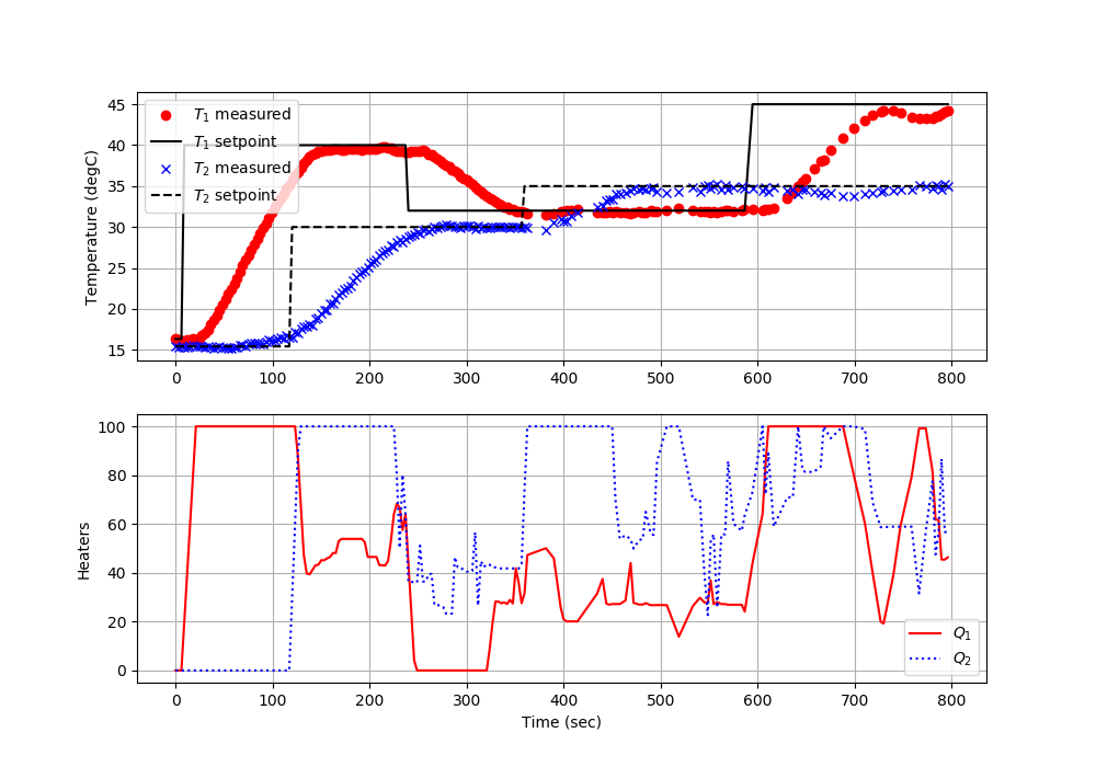
The TCLab is a hands-on application of machine learning and advanced temperature control with two heaters and two temperature sensors. The labs reinforce principles of model development, estimation, and advanced control methods. This is the sixth exercise and it involves linear model predictive control with an empirical 2nd order model. The predictions were previously aligned to the measured values through an estimator. This model predictive controller uses those parameters and a linear model of the TCLab input to output response to control temperatures to a set point.

See information on Model Predictive Control (MPC) and MPC Examples in Excel, MATLAB, Simulink, and Python.

Lab Problem Statement

• Lab F - Linear Model Predictive Control

Data and Solutions

• Solution with Python

(:html:) <iframe width="560" height="315" src="https://www.youtube.com/embed/P_tPc0LvHJY" frameborder="0" allow="accelerometer; autoplay; encrypted-media; gyroscope; picture-in-picture" allowfullscreen></iframe> (:htmlend:)

• Solution with MATLAB

(:html:) <iframe width="560" height="315" src="https://www.youtube.com/embed/7WMVUMM5Dt0" frameborder="0" allow="accelerometer; autoplay; encrypted-media; gyroscope; picture-in-picture" allowfullscreen></iframe> (:htmlend:)

(:toggle hide gekko_labF1 button show="Lab F: Python TCLab SISO MPC with 1st Order Model":) (:div id=gekko_labF1:) (:source lang=python:) import tclab import numpy as np import time import matplotlib.pyplot as plt from gekko import GEKKO

1. Connect to Arduino

a = tclab.TCLab()

1. Get Version

print(a.version)

1. Turn LED on

print('LED On') a.LED(100)

1. Run time in minutes

run_time = 5.0

1. Number of cycles

loops = int(60.0*run_time) tm = np.zeros(loops)

1. Temperature (K)

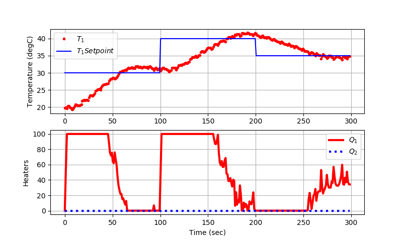
T1 = np.ones(loops) * a.T1 # temperature (degC) Tsp1 = np.ones(loops) * 30.0 # set point (degC)

1. Set point changes

Tsp1[100:] = 40.0 Tsp1[200:] = 35.0

T2 = np.ones(loops) * a.T2 # temperature (degC) Tsp2 = np.ones(loops) * 23.0 # set point (degC)

1. heater values

Q1s = np.ones(loops) * 0.0 Q2s = np.ones(loops) * 0.0

1. Initialize Model as Estimator

2. use remote=True for MacOS

m = GEKKO(name='tclab-mpc',remote=False)

1. 30 second time horizon

m.time = np.linspace(0,30,31)

1. Parameters

Q1_ss = m.Param(value=0) TC1_ss = m.Param(value=23) Kp = m.Param(value=0.4) tau = m.Param(value=160.0)

1. Manipulated variable

Q1 = m.MV(value=0) Q1.STATUS = 1 # use to control temperature Q1.FSTATUS = 0 # no feedback measurement Q1.LOWER = 0.0 Q1.UPPER = 100.0 Q1.DMAX = 50.0 Q1.COST = 0.0 Q1.DCOST = 1.0e-4

1. Controlled variable

TC1 = m.CV(value=TC1_ss) TC1.STATUS = 1 # minimize error with setpoint range TC1.FSTATUS = 1 # receive measurement TC1.TR_INIT = 2 # reference trajectory TC1.TAU = 10 # time constant for response

1. Equation

m.Equation(tau * TC1.dt() + (TC1-TC1_ss) == Kp * (Q1-Q1_ss))

1. Global Options

m.options.IMODE = 6 # MPC m.options.CV_TYPE = 1 # Objective type m.options.NODES = 3 # Collocation nodes m.options.SOLVER = 1 # 1=APOPT, 3=IPOPT

1. Create plot

plt.figure() plt.ion() plt.show()

1. Main Loop

start_time = time.time() prev_time = start_time try:

    for i in range(1,loops):
        # Sleep time
        sleep_max = 1.0
        sleep = sleep_max - (time.time() - prev_time)
        if sleep>=0.01:
            time.sleep(sleep)
        else:
            time.sleep(0.01)

        # Record time and change in time
        t = time.time()
        dt = t - prev_time
        prev_time = t
        tm[i] = t - start_time

        # Read temperatures in Kelvin 
        T1[i] = a.T1
        T2[i] = a.T2

        ###############################
        ### MPC CONTROLLER          ###
        ###############################
        TC1.MEAS = T1[i]
        # input setpoint with deadband +/- DT
        DT = 0.1
        TC1.SPHI = Tsp1[i] + DT
        TC1.SPLO = Tsp1[i] - DT
        # solve MPC
        m.solve(disp=False)    
        # test for successful solution
        if (m.options.APPSTATUS==1):
            # retrieve the first Q value
            Q1s[i] = Q1.NEWVAL
        else:
            # not successful, set heater to zero
            Q1s[i] = 0        

        # Write output (0-100)
        a.Q1(Q1s[i])
        a.Q2(Q2s[i])

        # Plot
        plt.clf()
        ax=plt.subplot(2,1,1)
        ax.grid()
        plt.plot(tm[0:i],T1[0:i],'ro',MarkerSize=3,label=r'$T_1$')
        plt.plot(tm[0:i],Tsp1[0:i],'b-',MarkerSize=3,label=r'$T_1 Setpoint$')
        plt.ylabel('Temperature (degC)')
        plt.legend(loc='best')
        ax=plt.subplot(2,1,2)
        ax.grid()
        plt.plot(tm[0:i],Q1s[0:i],'r-',LineWidth=3,label=r'$Q_1$')
        plt.plot(tm[0:i],Q2s[0:i],'b:',LineWidth=3,label=r'$Q_2$')
        plt.ylabel('Heaters')
        plt.xlabel('Time (sec)')
        plt.legend(loc='best')
        plt.draw()
        plt.pause(0.05)

    # Turn off heaters
    a.Q1(0)
    a.Q2(0)
    print('Shutting down')

1. Allow user to end loop with Ctrl-C

except KeyboardInterrupt:

    # Disconnect from Arduino
    a.Q1(0)
    a.Q2(0)
    print('Shutting down')
    a.close()

1. Make sure serial connection still closes when there's an error

except:

    # Disconnect from Arduino
    a.Q1(0)
    a.Q2(0)
    print('Error: Shutting down')
    a.close()
    raise

(:sourceend:) (:divend:)

(:toggle hide gekko_labF2 button show="Lab F: Python TCLab MIMO MPC with 2nd Order Model":) (:div id=gekko_labF2:) (:source lang=python:) import numpy as np import time import matplotlib.pyplot as plt import random

1. get gekko package with:
2. pip install gekko

from gekko import GEKKO

1. get tclab package with:
2. pip install tclab

from tclab import TCLab

1. Connect to Arduino

a = TCLab()

1. Final time

tf = 10 # min

1. number of data points (every 3 seconds)

n = tf * 20 + 1

1. Percent Heater (0-100%)

Q1s = np.zeros(n) Q2s = np.zeros(n)

1. Temperatures (degC)

T1m = a.T1 * np.ones(n) T2m = a.T2 * np.ones(n)

1. Temperature setpoints

T1sp = T1m[0] * np.ones(n) T2sp = T2m[0] * np.ones(n)

1. Heater set point steps about every 150 sec

T1sp[3:] = 40.0 T2sp[40:] = 30.0 T1sp[80:] = 32.0 T2sp[120:] = 35.0 T1sp[160:] = 45.0

1. Initialize Model as Estimator

2. use remote=True for MacOS

m = GEKKO(name='tclab-mpc',remote=False)

1. Control horizon, non-uniform time steps

m.time = [0,3,6,10,14,18,22,27,32,38,45,55,65, 75,90,110,130,150]

1. Parameters from Estimation

K1 = m.FV(value=0.607) K2 = m.FV(value=0.293) K3 = m.FV(value=0.24) tau12 = m.FV(value=192) tau3 = m.FV(value=15)

1. don't update parameters with optimizer

K1.STATUS = 0 K2.STATUS = 0 K3.STATUS = 0 tau12.STATUS = 0 tau3.STATUS = 0

1. Measured inputs

Q1 = m.MV(value=0) Q1.STATUS = 1 # manipulated Q1.FSTATUS = 0 # measured Q1.DMAX = 20.0 Q1.DCOST = 0.1 Q1.UPPER = 100.0 Q1.LOWER = 0.0

Q2 = m.MV(value=0) Q2.STATUS = 1 # manipulated Q2.FSTATUS = 0 # measured Q2.DMAX = 30.0 Q2.DCOST = 0.1 Q2.UPPER = 100.0 Q2.LOWER = 0.0

1. State variables

TH1 = m.SV(value=T1m[0]) TH2 = m.SV(value=T2m[0])

1. Measurements for model alignment

TC1 = m.CV(value=T1m[0]) TC1.STATUS = 1 # minimize error TC1.FSTATUS = 1 # receive measurement TC1.TAU = 10 # response speed (time constant) TC1.TR_INIT = 2 # reference trajectory

TC2 = m.CV(value=T2m[0]) TC2.STATUS = 1 # minimize error TC2.FSTATUS = 1 # receive measurement TC2.TAU = 10 # response speed (time constant) TC2.TR_INIT = 2 # reference trajectory

Ta = m.Param(value=23.0) # degC

1. Heat transfer between two heaters

DT = m.Intermediate(TH2-TH1)

1. Empirical correlations

m.Equation(tau12 * TH1.dt() + (TH1-Ta) == K1*Q1 + K3*DT) m.Equation(tau12 * TH2.dt() + (TH2-Ta) == K2*Q2 - K3*DT) m.Equation(tau3 * TC1.dt() + TC1 == TH1) m.Equation(tau3 * TC2.dt() + TC2 == TH2)

1. Global Options

m.options.IMODE = 6 # MHE m.options.EV_TYPE = 1 # Objective type m.options.NODES = 3 # Collocation nodes m.options.SOLVER = 3 # IPOPT m.options.COLDSTART = 1 # COLDSTART on first cycle

1. Create plot

plt.figure(figsize=(10,7)) plt.ion() plt.show()

1. Main Loop

start_time = time.time() prev_time = start_time tm = np.zeros(n)

try:

    for i in range(1,n):
        # Sleep time
        sleep_max = 3.0
        sleep = sleep_max - (time.time() - prev_time)
        if sleep>=0.01:
            time.sleep(sleep-0.01)
        else:
            time.sleep(0.01)

        # Record time and change in time
        t = time.time()
        dt = t - prev_time
        prev_time = t
        tm[i] = t - start_time

        # Read temperatures in Celsius 
        T1m[i] = a.T1
        T2m[i] = a.T2

        # Insert measurements
        TC1.MEAS = T1m[i]
        TC2.MEAS = T2m[i]

        # Adjust setpoints
        TC1.SPHI = T1sp[i] + 0.1
        TC1.SPLO = T1sp[i] - 0.1

        TC2.SPHI = T2sp[i] + 0.1
        TC2.SPLO = T2sp[i] - 0.1

        # Predict Parameters and Temperatures with MHE
        # use remote=False for local solve
        m.solve() 

        if m.options.APPSTATUS == 1:
            # Retrieve new values
            Q1s[i]  = Q1.NEWVAL
            Q2s[i]  = Q2.NEWVAL
        else:
            # Solution failed
            Q1s[i]  = 0.0
            Q2s[i]  = 0.0

        # Write new heater values (0-100)
        a.Q1(Q1s[i])
        a.Q2(Q2s[i])

        # Plot
        plt.clf()
        ax=plt.subplot(2,1,1)
        ax.grid()
        plt.plot(tm[0:i],T1m[0:i],'ro',label=r'$T_1$ measured')
        plt.plot(tm[0:i],T1sp[0:i],'k-',label=r'$T_1$ setpoint')
        plt.plot(tm[0:i],T2m[0:i],'bx',label=r'$T_2$ measured')
        plt.plot(tm[0:i],T2sp[0:i],'k--',label=r'$T_2$ setpoint')
        plt.ylabel('Temperature (degC)')
        plt.legend(loc=2)
        ax=plt.subplot(2,1,2)
        ax.grid()
        plt.plot(tm[0:i],Q1s[0:i],'r-',label=r'$Q_1$')
        plt.plot(tm[0:i],Q2s[0:i],'b:',label=r'$Q_2$')
        plt.ylabel('Heaters')
        plt.xlabel('Time (sec)')
        plt.legend(loc='best')
        plt.draw()
        plt.pause(0.05)

    # Turn off heaters and close connection
    a.Q1(0)
    a.Q2(0)
    a.close()
    # Save figure
    plt.savefig('tclab_mpc.png')

1. Allow user to end loop with Ctrl-C

except KeyboardInterrupt:

    # Turn off heaters and close connection
    a.Q1(0)
    a.Q2(0)
    a.close()
    print('Shutting down')
    plt.savefig('tclab_mpc.png')

1. Make sure serial connection still closes when there's an error

except:

    # Disconnect from Arduino
    a.Q1(0)
    a.Q2(0)
    a.close()
    print('Error: Shutting down')
    plt.savefig('tclab_mpc.png')
    raise

(:sourceend:) (:divend:)

See also:

Advanced Control Lab Overview

GEKKO Documentation

TCLab Documentation

TCLab Files on GitHub

Basic (PID) Control Lab

(:html:) <style> .button {

  border-radius: 4px;
  background-color: #0000ff;
  border: none;
  color: #FFFFFF;
  text-align: center;
  font-size: 28px;
  padding: 20px;
  width: 300px;
  transition: all 0.5s;
  cursor: pointer;
  margin: 5px;

}

.button span {

  cursor: pointer;
  display: inline-block;
  position: relative;
  transition: 0.5s;

}

.button span:after {

  content: '\00bb';
  position: absolute;
  opacity: 0;
  top: 0;
  right: -20px;
  transition: 0.5s;

}

.button:hover span {

  padding-right: 25px;

}

.button:hover span:after {

  opacity: 1;
  right: 0;

} </style> (:htmlend:)