TCLab B - MIMO Digital Twin
Main.TCLabB History
Hide minor edits - Show changes to markup
Virtual TCLab on Google Colab
(:title TCLab B - MIMO Modeling:)
(:title TCLab B - MIMO Digital Twin:)
GEKKO Documentation
TCLab Documentation
(:title TCLab B - MIMO Modeling:) (:keywords Arduino, PID, temperature, control, process control, course:) (:description Multivariate (MIMO) Energy Balance and Deep Learning with Arduino Data from TCLab:)
The TCLab is a hands-on application of machine learning and advanced temperature control with two heaters and two temperature sensors. The labs reinforce principles of model development, estimation, and advanced control methods. This is the second exercise to simulate an energy balance and compare the predictions to deep learning with a multi-layered neural network. The additional feature over the first lab is that the model is extended to two heaters and two temperature sensors.
Lab Problem Statement
Data and Solutions
Lab B
(:html:) <iframe width="560" height="315" src="https://www.youtube.com/embed/ZUHiQORwmxw" frameborder="0" allow="autoplay; encrypted-media" allowfullscreen></iframe> (:htmlend:)
- MIMO Energy Balance Solution with MATLAB and Python
- Steady state data, 2 heaters
- Dynamic data, 2 heaters
(:toggle hide gekko_labBd button show="Lab B: Python TCLab Generate Step Data":) (:div id=gekko_labBd:) (:source lang=python:) import numpy as np import pandas as pd import tclab import time import matplotlib.pyplot as plt
- generate step test data on Arduino
filename = 'tclab_dyn_data2.csv'
- heater steps
Q1d = np.zeros(601) Q1d[10:200] = 80 Q1d[200:280] = 20 Q1d[280:400] = 70 Q1d[400:] = 50
Q2d = np.zeros(601) Q2d[120:320] = 100 Q2d[320:520] = 10 Q2d[520:] = 80
- Connect to Arduino
a = tclab.TCLab() fid = open(filename,'w') fid.write('Time,H1,H2,T1,T2\n') fid.close()
- run step test (10 min)
for i in range(601):
    # set heater values
    a.Q1(Q1d[i])
    a.Q2(Q2d[i])
    print('Time: ' + str(i) +           ' H1: ' + str(Q1d[i]) +           ' H2: ' + str(Q2d[i]) +           ' T1: ' + str(a.T1)   +           ' T2: ' + str(a.T2))
    # wait 1 second
    time.sleep(1)
    fid = open(filename,'a')
    fid.write(str(i)+',str(Q1d[i]),str(Q2d[i]),'               +str(a.T1)+',str(a.T2)\n')
- close connection to Arduino
a.close()
- read data file
data = pd.read_csv(filename)
- plot measurements
plt.figure() plt.subplot(2,1,1) plt.plot(data['Time'],data['H1'],'r-',label='Heater 1') plt.plot(data['Time'],data['H2'],'b--',label='Heater 2') plt.ylabel('Heater (%)') plt.legend(loc='best') plt.subplot(2,1,2) plt.plot(data['Time'],data['T1'],'r.',label='Temperature 1') plt.plot(data['Time'],data['T2'],'b.',label='Temperature 2') plt.ylabel('Temperature (degC)') plt.legend(loc='best') plt.xlabel('Time (sec)') plt.savefig('tclab_dyn_meas2.png')
plt.show() (:sourceend:) (:divend:)
(:toggle hide gekko_labBf button show="Lab B: Python GEKKO Energy Balance":) (:div id=gekko_labBf:)
(:source lang=python:) import numpy as np import matplotlib.pyplot as plt from gekko import GEKKO
- initialize GEKKO model
m = GEKKO()
- model discretized time
n = 60*10+1 # Number of second time points (10min) m.time = np.linspace(0,n-1,n) # Time vector
- Parameters
- Percent Heater (0-100%)
Q1d = np.zeros(n) Q1d[10:200] = 80 Q1d[200:280] = 20 Q1d[280:400] = 70 Q1d[400:] = 50 Q1 = m.Param() Q1.value = Q1d
Q2d = np.zeros(n) Q2d[120:320] = 100 Q2d[320:520] = 10 Q2d[520:] = 80 Q2 = m.Param() Q2.value = Q2d# Heaters as time-varying inputs Q1 = m.Param(value=Q1d) # Percent Heater (0-100%) Q2 = m.Param(value=Q2d) # Percent Heater (0-100%)
T0 = m.Param(value=19.0+273.15) # Initial temperature Ta = m.Param(value=19.0+273.15) # K U = m.Param(value=10.0) # W/m^2-K mass = m.Param(value=4.0/1000.0) # kg Cp = m.Param(value=0.5*1000.0) # J/kg-K A = m.Param(value=10.0/100.0**2) # Area not between heaters in m^2 As = m.Param(value=2.0/100.0**2) # Area between heaters in m^2 alpha1 = m.Param(value=0.01) # W / % heater alpha2 = m.Param(value=0.005) # W / % heater eps = m.Param(value=0.9) # Emissivity sigma = m.Const(5.67e-8) # Stefan-Boltzman
- Temperature states as GEKKO variables
T1 = m.Var(value=T0) T2 = m.Var(value=T0)
- Between two heaters
Q_C12 = m.Intermediate(U*As*(T2-T1)) # Convective Q_R12 = m.Intermediate(eps*sigma*As*(T2**4-T1**4)) # Radiative
m.Equation(T1.dt() == (1.0/(mass*Cp))*(U*A*(Ta-T1) + eps * sigma * A * (Ta**4 - T1**4) + Q_C12 + Q_R12 + alpha1*Q1))
m.Equation(T2.dt() == (1.0/(mass*Cp))*(U*A*(Ta-T2) + eps * sigma * A * (Ta**4 - T2**4) - Q_C12 - Q_R12 + alpha2*Q2))
- simulation mode
m.options.IMODE = 4
- simulation model
m.solve()
- plot results
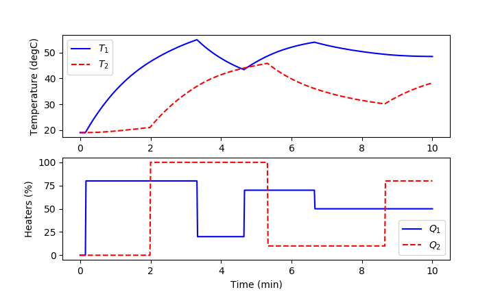
plt.figure(1) plt.subplot(2,1,1) plt.plot(m.time/60.0,np.array(T1.value)-273.15,'b-') plt.plot(m.time/60.0,np.array(T2.value)-273.15,'r--') plt.legend([r'$T_1$',r'$T_2$'],loc='best') plt.ylabel('Temperature (degC)')
plt.subplot(2,1,2) plt.plot(m.time/60.0,np.array(Q1.value),'b-') plt.plot(m.time/60.0,np.array(Q2.value),'r--') plt.legend([r'$Q_1$',r'$Q_2$'],loc='best') plt.ylabel('Heaters (%)')
plt.xlabel('Time (min)') plt.show() (:sourceend:) (:divend:)
(:toggle hide gekko_labBnn button show="Lab B: Python GEKKO Neural Network":) (:div id=gekko_labBnn:)
(:source lang=python:) import numpy as np import pandas as pd import matplotlib.pyplot as plt from sklearn.preprocessing import MinMaxScaler from gekko import GEKKO
import time
- -------------------------------------
- import or generate data
- -------------------------------------
filename = 'tclab_ss_data2.csv' try:
    try:
        data = pd.read_csv(filename)
    except:
        url = 'https://apmonitor.com/do/uploads/Main/tclab_ss_data2.txt'
        data = pd.read_csv(url)
except:
    # generate training data if data file not available
    import tclab
    # Connect to Arduino
    a = tclab.TCLab()
    fid = open(filename,'w')
    fid.write('Heater 1,Heater 2,Temperature 1,Temperature 2\n')
    fid.close()
    # data collection takes 6 hours = 120 pts * 3 minutes each
    npts = 120
    for i in range(npts):
        # set random heater values
        Q1 = np.random.rand()*100
        Q2 = np.random.rand()*100
        a.Q1(Q1)
        a.Q2(Q2)
        print('Heater 1: ' + str(Q1) + ' %')
        print('Heater 2: ' + str(Q2) + ' %')
        # wait 3 minutes
        time.sleep(3*60)
        # record temperature and heater value
        print('Temperature 1: ' + str(a.T1) + ' degC')
        print('Temperature 2: ' + str(a.T2) + ' degC')
        fid = open(filename,'a')
        fid.write(str(Q1)+',str(Q2),str(a.T1),str(a.T2)\n')
        fid.close()
    # close connection to Arduino
    a.close()
    # read data file
    data = pd.read_csv(filename)
- -------------------------------------
- scale data
- -------------------------------------
s = MinMaxScaler(feature_range=(0,1)) sc_train = s.fit_transform(data)
- partition into inputs and outputs
xs = sc_train[:,0:2] # 2 heaters ys = sc_train[:,2:4] # 2 temperatures
- -------------------------------------
- build neural network
- -------------------------------------
nin = 2 # inputs n1 = 2 # hidden layer 1 (linear) n2 = 2 # hidden layer 2 (nonlinear) n3 = 2 # hidden layer 3 (linear) nout = 2 # outputs
- Initialize gekko models
train = GEKKO() dyn = GEKKO() model = [train,dyn]
for m in model:
    # use APOPT solver
    m.options.SOLVER = 1

    # input(s)
    m.inpt = [m.Param() for i in range(nin)]

    # layer 1 (linear)
    m.w1 = m.Array(m.FV, (nout,nin,n1))
    m.l1 = [[m.Intermediate(sum([m.w1[k,j,i]*m.inpt[j]             for j in range(nin)])) for i in range(n1)]             for k in range(nout)]

    # layer 2 (tanh)
    m.w2 = m.Array(m.FV, (nout,n1,n2))
    m.l2 = [[m.Intermediate(sum([m.tanh(m.w2[k,j,i]*m.l1[k][j])             for j in range(n1)])) for i in range(n2)]             for k in range(nout)]

    # layer 3 (linear)
    m.w3 = m.Array(m.FV, (nout,n2,n3))
    m.l3 = [[m.Intermediate(sum([m.w3[k,j,i]*m.l2[k][j]             for j in range(n2)])) for i in range(n3)]             for k in range(nout)]

    # outputs
    m.outpt = [m.CV() for i in range(nout)]
    m.Equations([m.outpt[k]==sum([m.l3[k][i] for i in range(n3)])                  for k in range(nout)])

    # flatten matrices
    m.w1 = m.w1.flatten()
    m.w2 = m.w2.flatten()
    m.w3 = m.w3.flatten()
- -------------------------------------
- fit parameter weights
- -------------------------------------
m = train for i in range(nin):
m.inpt[i].value=xs[:,i]
for i in range(nout):
    m.outpt[i].value = ys[:,i]
    m.outpt[i].FSTATUS = 1
for i in range(len(m.w1)):
    m.w1[i].FSTATUS=1
    m.w1[i].STATUS=1
    m.w1[i].MEAS=1.0
for i in range(len(m.w2)):
    m.w2[i].STATUS=1
    m.w2[i].FSTATUS=1
    m.w2[i].MEAS=0.5
for i in range(len(m.w3)):
    m.w3[i].FSTATUS=1
    m.w3[i].STATUS=1
    m.w3[i].MEAS=1.0
m.options.IMODE = 2 m.options.EV_TYPE = 2
- solve for weights to minimize loss (objective)
m.solve(disp=True)
- -------------------------------------
- generate dynamic predictions
- -------------------------------------
m = dyn tf = 600 m.time = np.linspace(0,tf,tf+1)
- load neural network parameters
for i in range(len(m.w1)):
    m.w1[i].MEAS=train.w1[i].NEWVAL
    m.w1[i].FSTATUS = 1
for i in range(len(m.w2)):
    m.w2[i].MEAS=train.w2[i].NEWVAL
    m.w2[i].FSTATUS = 1
for i in range(len(m.w3)):
    m.w3[i].MEAS=train.w3[i].NEWVAL
    m.w3[i].FSTATUS = 1
- step tests
Q1d = np.zeros(tf+1) Q1d[10:200] = 80 Q1d[200:280] = 20 Q1d[280:400] = 70 Q1d[400:] = 50 Q1 = m.Param() Q1.value = Q1d
Q2d = np.zeros(tf+1) Q2d[120:320] = 100 Q2d[320:520] = 10 Q2d[520:] = 80 Q2 = m.Param() Q2.value = Q2d
- scaled inputs
m.inpt[0].value = Q1d * s.scale_[0] + s.min_[0] m.inpt[1].value = Q2d * s.scale_[1] + s.min_[1]
- define Temperature output
Q0 = 0 # initial heater T0 = 19 # ambient temperature
- scaled steady state ouput
T1_ss = m.Var(value=T0) T2_ss = m.Var(value=T0) m.Equation(T1_ss == (m.outpt[0]-s.min_[2])/s.scale_[2]) m.Equation(T2_ss == (m.outpt[1]-s.min_[3])/s.scale_[3])
- dynamic prediction
T1 = m.Var(value=T0) T2 = m.Var(value=T0)
- time constant
tau = m.Param(value=120) # determine in a later exercise
- additional model equation for dynamics
m.Equation(tau*T1.dt()==-(T1-T0)+(T1_ss-T0)) m.Equation(tau*T2.dt()==-(T2-T0)+(T2_ss-T0))
- solve dynamic simulation
m.options.IMODE=4 m.solve()
- generate step test data on Arduino
- -------------------------------------
- import or generate data
- -------------------------------------
filename = 'tclab_dyn_data2.csv' try:
    try:
        data = pd.read_csv(filename)
    except:
        url = 'https://apmonitor.com/do/uploads/Main/tclab_dyn_data2.txt'
        data = pd.read_csv(url)
except:
    # generate training data if data file not available
    import tclab
    # Connect to Arduino
    a = tclab.TCLab()
    fid = open(filename,'w')
    fid.write('Time,H1,H2,T1,T2\n')
    fid.close()
    # check for cool down
    i = 0
    while i<=10:
        i += 1 # upper limit on wait time
        T1m = a.T1
        T2m = a.T2
        print('T1: ' + str(a.T1) + ' T2: ' + str(a.T2))
        print('Sleep 30 sec')
        time.sleep(30)
        if (a.T1<30 and a.T2<30 and a.T1>=T1m-0.2 and a.T2>=T2m-0.2):
            break  # continue when conditions met
        else:
            print('Not at ambient temperature')
    # run step test (10 min)
    for i in range(tf+1):
        # set heater values
        a.Q1(Q1d[i])
        a.Q2(Q2d[i])
        print('Time: ' + str(i) +               ' H1: ' + str(Q1d[i]) +               ' H2: ' + str(Q2d[i]) +               ' T1: ' + str(a.T1)   +               ' T2: ' + str(a.T2))
        # wait 1 second
        time.sleep(1)
        fid = open(filename,'a')
        fid.write(str(i)+',str(Q1d[i]),str(Q2d[i]),'                   +str(a.T1)+',str(a.T2)\n')
        fid.close()
    # close connection to Arduino
    a.close()
    # read data file
    data = pd.read_csv(filename)
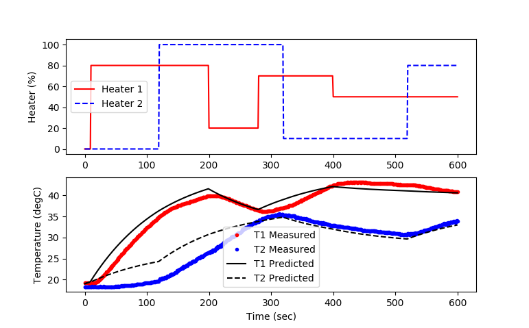
- plot prediction and measurement
plt.figure() plt.subplot(2,1,1) plt.plot(m.time,Q1.value,'r-',label='Heater 1') plt.plot(m.time,Q2.value,'b--',label='Heater 2') plt.ylabel('Heater (%)') plt.legend(loc='best') plt.subplot(2,1,2) plt.plot(data['Time'],data['T1'],'r.',label='T1 Measured') plt.plot(data['Time'],data['T2'],'b.',label='T2 Measured') plt.plot(m.time,T1.value,'k-',label='T1 Predicted') plt.plot(m.time,T2.value,'k--',label='T2 Predicted') plt.ylabel('Temperature (degC)') plt.legend(loc='best') plt.xlabel('Time (sec)') plt.savefig('tclab_dyn_pred.png')
plt.show() (:sourceend:) (:divend:)
See also:
Advanced Control Lab Overview
TCLab Files on GitHub Basic (PID) Control Lab
(:html:) <style> .button {
  border-radius: 4px;
  background-color: #0000ff;
  border: none;
  color: #FFFFFF;
  text-align: center;
  font-size: 28px;
  padding: 20px;
  width: 300px;
  transition: all 0.5s;
  cursor: pointer;
  margin: 5px;
}
.button span {
  cursor: pointer;
  display: inline-block;
  position: relative;
  transition: 0.5s;
}
.button span:after {
  content: '\00bb';
  position: absolute;
  opacity: 0;
  top: 0;
  right: -20px;
  transition: 0.5s;
}
.button:hover span {
padding-right: 25px;
}
.button:hover span:after {
  opacity: 1;
  right: 0;
} </style> (:htmlend:)