Dynamic Optimization

1. animate plot?

animate=False

data = pd.read_csv(file2)

plt.figure(figsize=(12,8))

if animate:

    plt.ion()
    plt.show()
    make_gif = True
    try:
        import imageio  # required to make gif animation
    except:
        print('install imageio with "pip install imageio" to make gif')
        make_gif=False
    if make_gif:
        try:
            import os
            images = []
            os.mkdir('./frames')
        except:
            print('Figure directory already created')

plt.legend(loc=3)

plt.legend(loc=3)

plt.legend(loc=3)

if animate:

    t = data['Time'].values/60
    n = len(t)
    for i in range(60,n+1,10):
        for j in range(3):
            plt.subplot(gs[j])
            plt.xlim([t[max(0,i-1200)],t[i]])        
        filename='./frames/frame_str(1000+i).png'
        plt.savefig(filename)
        if make_gif:
            images.append(imageio.imread(filename))
        plt.pause(0.1)

    # create animated GIF
    if make_gif:
        imageio.mimsave('animate.gif', images)
        imageio.mimsave('animate.mp4', images)

else:

    plt.show()

(:html:) <video width="550" controls autoplay loop>

  <source src="/do/uploads/Main/tclab_classifiers.mp4" type="video/mp4">
  Your browser does not support the video tag.

</video> (:htmlend:)

(:html:) <iframe width="560" height="315" src="https://www.youtube.com/embed/OzkmOTq5zq4" frameborder="0" allow="accelerometer; autoplay; encrypted-media; gyroscope; picture-in-picture" allowfullscreen></iframe> (:htmlend:)

Disadvantages: Assumes all predictors are independent of each other, and assumes data is free of missing values.

(:toggle hide svm button show="Number Identification with SVM":) (:div id=svm:)

plt.show() (:sourceend:) (:divend:)

(:toggle hide class8 button show="Number Identification with 8 Classifiers":) (:div id=class8:) (:source lang=python:) from sklearn import datasets, metrics from sklearn.model_selection import train_test_split import matplotlib.pyplot as plt import numpy as np import time

1. The digits dataset

digits = datasets.load_digits() n_samples = len(digits.images) data = digits.images.reshape((n_samples, -1))

1. Split into train and test subsets (50% each)

XA, XB, yA, yB = train_test_split(

    data, digits.target, test_size=0.5, shuffle=False)

1. Logistic Regression

from sklearn.linear_model import LogisticRegression lr = LogisticRegression(solver='lbfgs',multi_class='auto',max_iter=2000)

1. Naïve Bayes

from sklearn.naive_bayes import GaussianNB nb = GaussianNB()

1. Stochastic Gradient Descent

from sklearn.linear_model import SGDClassifier sgd = SGDClassifier(loss='modified_huber', shuffle=True,random_state=101, tol=1e-3,max_iter=1000)

1. K-Nearest Neighbors

from sklearn.neighbors import KNeighborsClassifier knn = KNeighborsClassifier(n_neighbors=10)

1. Decision Tree

from sklearn.tree import DecisionTreeClassifier dtree = DecisionTreeClassifier(max_depth=10,random_state=101, max_features=None,min_samples_leaf=5)

1. Random Forest

from sklearn.ensemble import RandomForestClassifier rfm = RandomForestClassifier(n_estimators=70,oob_score=True,n_jobs=1, random_state=101,max_features=None,min_samples_leaf=3)

1. Support Vector Classifier

from sklearn.svm import SVC svm = SVC(gamma='scale', C=1.0, random_state=101)

1. Neural Network

from sklearn.neural_network import MLPClassifier nn = MLPClassifier(solver='lbfgs',alpha=1e-5,max_iter=200, activation='relu',hidden_layer_sizes=(10,30,10), random_state=1, shuffle=True)

1. classification methods

m = [nb,lr,sgd,knn,dtree,rfm,svm,nn] s = ['nb','lr','sgd','knn','dt','rfm','svm','nn']

1. fit classifiers

print('Train Classifiers') for i,x in enumerate(m):

    st = time.time()
    x.fit(XA,yA)
    tf = str(round(time.time()-st,5))
    print(s[i] + ' time: ' + tf)

1. test on random number in second half of data

n = np.random.randint(int(n_samples/2),n_samples) Xt = digits.data[n:n+1]

1. test classifiers

print('Test Classifiers') for i,x in enumerate(m):

    st = time.time()
    yt = x.predict(Xt)
    tf = str(round(time.time()-st,5))
    print(s[i] + ' predicts: ' + str(yt[0]) + ' time: ' + tf)

print('Label: ' + str(digits.target[n:n+1][0]))

plt.imshow(digits.images[n], cmap=plt.cm.gray_r, interpolation='nearest') plt.show()

(:toggle hide tclab_sol button show="Show Solution with Source Code":)

Solutions

Select and scale (0-1) the features of the data such as temperature, and temperature derivatives. Use the measured temperature and derivatives and heater value labels to create a classifier that predicts when the heater is on or off. Validate the classifier with new data that was not used for training.

Solutions'

(:toggle hide tclab_sol button show="Solution Source Code":) (:div id=tclab_sol:)

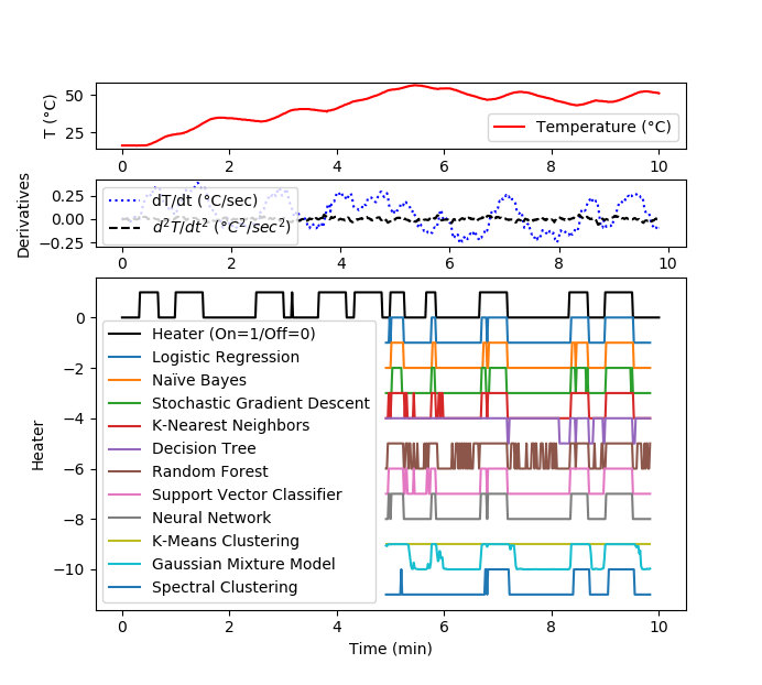
Solution for 10 minute data set

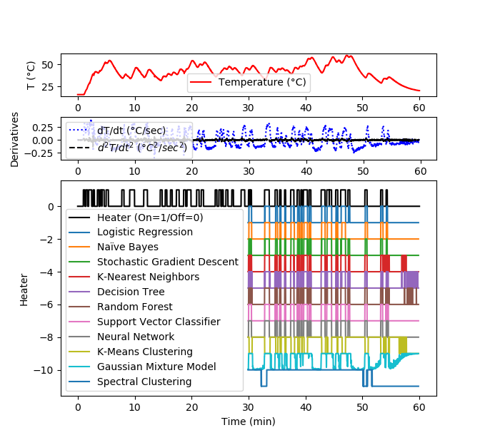
Solution for 1 hour data set

(:source lang=python:) import pandas as pd import numpy as np import matplotlib.pyplot as plt from matplotlib import gridspec from sklearn.preprocessing import MinMaxScaler from sklearn.model_selection import train_test_split

1. Load data

file1 = 'https://apmonitor.com/do/uploads/Main/tclab_data5.txt' file2 = 'https://apmonitor.com/do/uploads/Main/tclab_data6.txt' data = pd.read_csv(file1)

1. Input Features: Temperature and 1st / 2nd Derivatives
2. Cubic polynomial fit of temperature using 10 data points

data['dT1'] = np.zeros(len(data)) data['d2T1'] = np.zeros(len(data)) for i in range(len(data)):

    if i<len(data)-10:
        x = data['Time'][i:i+10]-data['Time'][i]
        y = data['T1'][i:i+10]
        p = np.polyfit(x,y,3)
        # evaluate derivatives at mid-point (5 sec)
        t = 5.0
        data['dT1'][i] = 3.0*p[0]*t**2 + 2.0*p[1]*t+p[2]
        data['d2T1'][i] = 6.0*p[0]*t + 2.0*p[1]
    else:
        data['dT1'][i] = np.nan
        data['d2T1'][i] = np.nan

1. Remove last 10 values

X = np.array(data'T1','dT1','d2T1'?[0:-10]) y = np.array(data'Q1'?[0:-10])

1. Scale data
2. Input features (Temperature and 2nd derivative at 5 sec)

s1 = MinMaxScaler(feature_range=(0,1)) Xs = s1.fit_transform(X)

1. Output labels (heater On / Off)

ys = [True if y[i]>50.0 else False for i in range(len(y))]

1. Split into train and test subsets (50% each)

XA, XB, yA, yB = train_test_split(Xs, ys, test_size=0.5, shuffle=False)

1. Plot regression results

def assess(P):

    plt.figure()
    plt.scatter(XB[P==1,0],XB[P==1,1],marker='^',color='blue',label='True')
    plt.scatter(XB[P==0,0],XB[P==0,1],marker='x',color='red',label='False')
    plt.scatter(XB[P!=yB,0],XB[P!=yB,1],marker='s',color='orange',                alpha=0.5,label='Incorrect')
    plt.legend()

1. Supervised Classification
2. Logistic Regression

from sklearn.linear_model import LogisticRegression lr = LogisticRegression(solver='lbfgs') lr.fit(XA,yA) yP1 = lr.predict(XB)

1. assess(yP1)
2. Naïve Bayes

from sklearn.naive_bayes import GaussianNB nb = GaussianNB() nb.fit(XA,yA) yP2 = nb.predict(XB)

1. assess(yP2)
2. Stochastic Gradient Descent

from sklearn.linear_model import SGDClassifier sgd = SGDClassifier(loss='modified_huber', shuffle=True,random_state=101) sgd.fit(XA,yA) yP3 = sgd.predict(XB)

1. assess(yP3)
2. K-Nearest Neighbors

from sklearn.neighbors import KNeighborsClassifier knn = KNeighborsClassifier(n_neighbors=5) knn.fit(XA,yA) yP4 = knn.predict(XB)

1. assess(yP4)
2. Decision Tree

from sklearn.tree import DecisionTreeClassifier dtree = DecisionTreeClassifier(max_depth=10,random_state=101, max_features=None,min_samples_leaf=5) dtree.fit(XA,yA) yP5 = dtree.predict(XB)

1. assess(yP5)
2. Random Forest

from sklearn.ensemble import RandomForestClassifier rfm = RandomForestClassifier(n_estimators=70,oob_score=True,n_jobs=1, random_state=101,max_features=None,min_samples_leaf=3) rfm.fit(XA,yA) yP6 = rfm.predict(XB)

1. assess(yP6)
2. Support Vector Classifier

from sklearn.svm import SVC svm = SVC(gamma='scale', C=1.0, random_state=101) svm.fit(XA,yA) yP7 = svm.predict(XB)

1. assess(yP7)
2. Neural Network

from sklearn.neural_network import MLPClassifier clf = MLPClassifier(solver='lbfgs',alpha=1e-5,max_iter=200, activation='relu',hidden_layer_sizes=(10,30,10), random_state=1, shuffle=True) clf.fit(XA,yA) yP8 = clf.predict(XB)

1. assess(yP8)
2. Unsupervised Classification
3. K-Means Clustering

from sklearn.cluster import KMeans km = KMeans(n_clusters=2) km.fit(XA) yP9 = km.predict(XB)

1. Arbitrary labels with unsupervised clustering may need to be reversed
2. yP9 = 1.0-yP9
3. assess(yP9)
4. Gaussian Mixture Model

from sklearn.mixture import GaussianMixture gmm = GaussianMixture(n_components=2) gmm.fit(XA) yP10 = gmm.predict_proba(XB) # produces probabilities

1. Arbitrary labels with unsupervised clustering may need to be reversed

yP10 = 1.0-yP10[:,0]

1. Spectral Clustering

from sklearn.cluster import SpectralClustering sc = SpectralClustering(n_clusters=2,eigen_solver='arpack', affinity='nearest_neighbors') yP11 = sc.fit_predict(XB) # No separation between fit and predict calls

                        #  need to fit and predict on same dataset

1. Arbitrary labels with unsupervised clustering may need to be reversed
2. yP11 = 1.0-yP11
3. assess(yP11)

plt.figure(1) gs = gridspec.GridSpec(3, 1, height_ratios=[1,1,5]) plt.subplot(gs[0]) plt.plot(data['Time']/60,data['T1'],'r-', label='Temperature (°C)') plt.ylabel('T (°C)') plt.legend() plt.subplot(gs[1]) plt.plot(data['Time']/60,data['dT1'],'b:', label='dT/dt (°C/sec)') plt.plot(data['Time']/60,data['d2T1'],'k--', label=r'$d^2T/dt^2$ ($°C^2/sec^2$)') plt.ylabel('Derivatives') plt.legend()

plt.subplot(gs[2]) plt.plot(data['Time']/60,data['Q1']/100,'k-', label='Heater (On=1/Off=0)')

t2 = data['Time'][len(yA):-10].values plt.plot(t2/60,yP1-1,label='Logistic Regression') plt.plot(t2/60,yP2-2,label='Naïve Bayes') plt.plot(t2/60,yP3-3,label='Stochastic Gradient Descent') plt.plot(t2/60,yP4-4,label='K-Nearest Neighbors') plt.plot(t2/60,yP5-5,label='Decision Tree') plt.plot(t2/60,yP6-6,label='Random Forest') plt.plot(t2/60,yP7-7,label='Support Vector Classifier') plt.plot(t2/60,yP8-8,label='Neural Network') plt.plot(t2/60,yP9-9,label='K-Means Clustering') plt.plot(t2/60,yP10-10,label='Gaussian Mixture Model') plt.plot(t2/60,yP11-11,label='Spectral Clustering')

plt.ylabel('Heater') plt.legend()

plt.xlabel(r'Time (min)') plt.legend() plt.show() (:sourceend:) (:divend:)

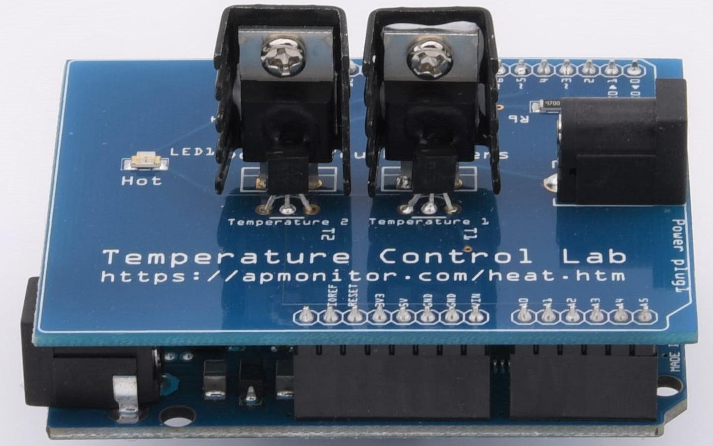
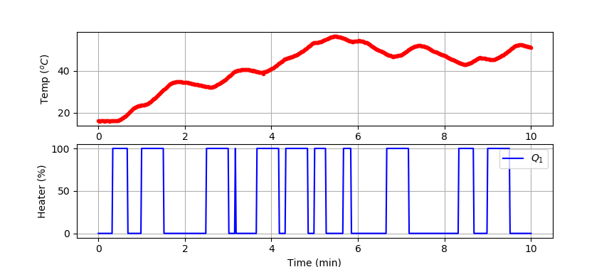
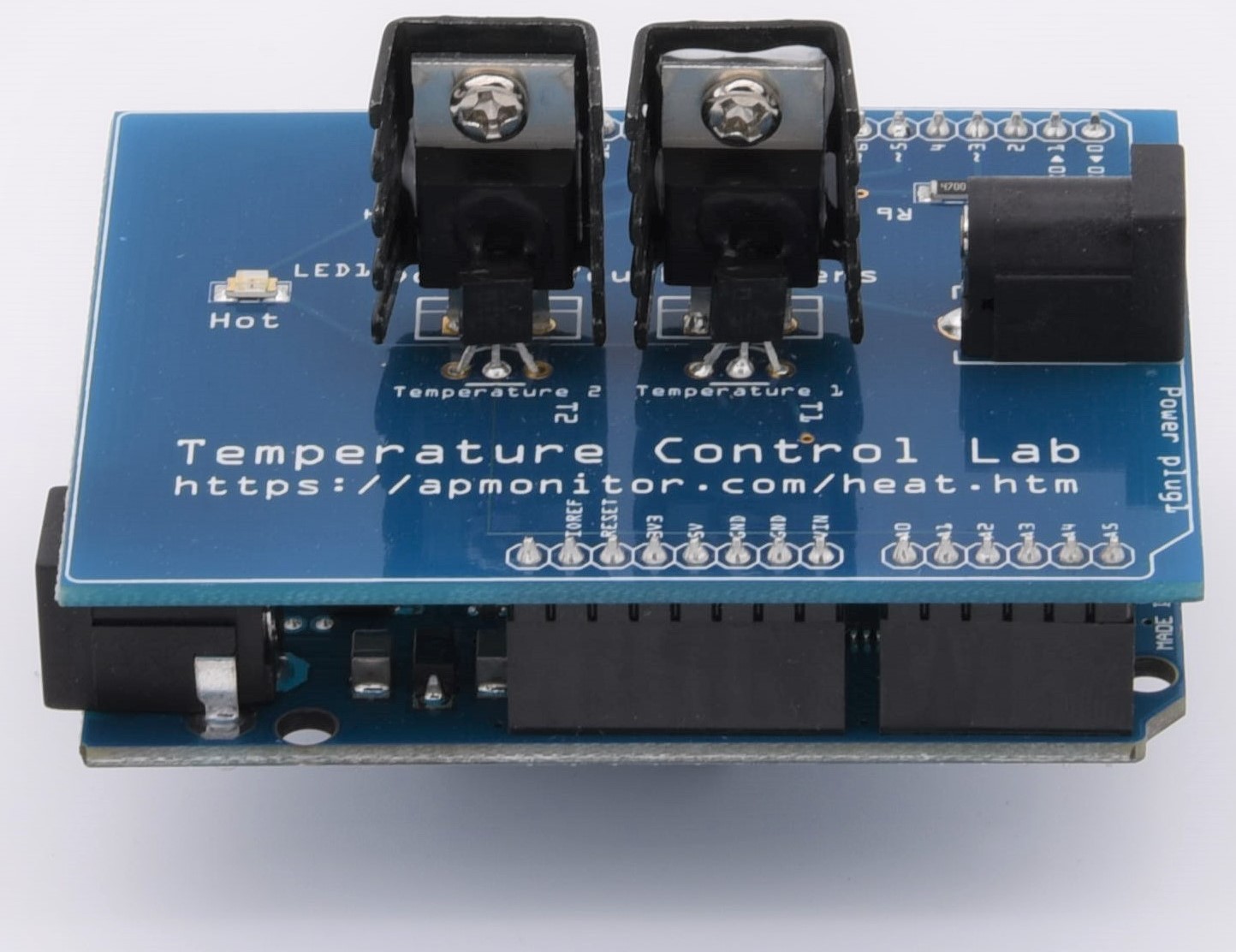
Develop a classifier to predict when the TCLab heater is on and when it is off. Generate labeled data where the heater is either on at 100% output or at 0% output for periods between 10 and 25 seconds.

Solutions

Small Data Set (10 min)

We test the classifier by splitting the data set into a training and test set. The data is generated from a TCLab or accessed at the link below.

Data for Testing

(:toggle hide tclab_test button show="Generate New TCLab Data for Testing (10 min)":) (:div id=tclab_test:)

n = 600 # Number of second time points (10 min)

Q1[20:41] = 100.0 Q1[60:91] = 100.0 Q1[150:181] = 100.0 Q1[190:206] = 100.0 Q1[220:251] = 100.0 Q1[260:291] = 100.0 Q1[300:316] = 100.0 Q1[340:351] = 100.0 Q1[400:431] = 100.0 Q1[500:521] = 100.0 Q1[540:571] = 100.0

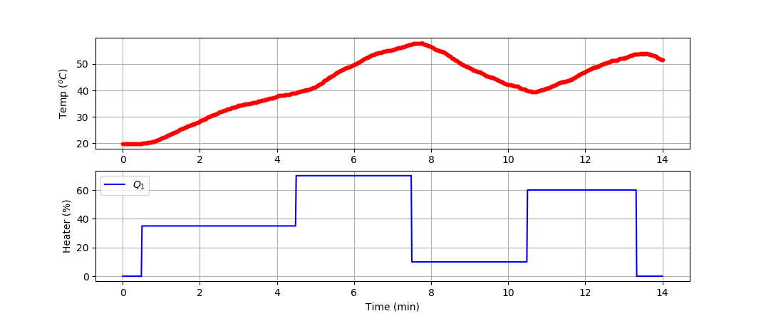
Large Data Set (1 hr)

Data for Training

(:toggle hide tclab_large button show="Generate New TCLab Data for Training (1 hr)":) (:div id=tclab_large:)

n = 3600 # Number of second time points (60 min)

1. random duration on (10-30 sec) in 60 second window
2. cool down last 5 minutes

k = 60 for i in range(1,n-301):

    if (i%k)==0:
        j = np.random.randint(10,26)
        k = np.random.randint(5,180)
        Q1[i:i+j+1] = 100.0

We select and scale (0-1) the features of the data such as temperature, and temperature derivatives.

Use the measured temperature and derivatives and heater value labels to create a classifier that predicts when the heater is on or off. We validate the classifier with new data that was not used for training.

K-Nearest Neighbors

Definition: Neighbors based classification is a type of lazy learning as it does not attempt to construct a general internal model, but simply stores instances of the training data. Classification is computed from a simple majority vote of the k nearest neighbors of each point.

1. K-Nearest Neighbors

Use the measured temperature and heater values to create a classifier that predicts when the heater is on or off. Validate the classifier with new data that was not used for training.

Solution

Develop a classifier to predict when the TCLab heater is on and when it is off. Generate labeled data where the heater is either on at 100% output or at 0% output for periods between 10 and 25 seconds or use the following training data.

Training Data

Test Data

Test the classifier on different data than was used for training. The data can be generated from a TCLab or accessed at the link below.

Develop a classifier to predict when the TCLab heater is on and when it is off. Generate labeled data where the heater is either on at 100% output or at 0% output for periods between 10 and 25 seconds.

Develop a classifier to predict when the TCLab heater is on. Generate labeled data where the heater is either on at 100% output or at 0% output for periods between 10 and 25 seconds.

Data for Training Δ

(:toggle hide tclab_train button show="Generate New TCLab Data for Training (1 hr)":) (:div id=tclab_train:)

(:source lang=python:)

1. generate new data

import numpy as np import matplotlib.pyplot as plt import pandas as pd import tclab import time

n = 3600 # Number of second time points (60 min) tm = np.linspace(0,n,n+1) # Time values lab = tclab.TCLab() T1 = [lab.T1] T2 = [lab.T2] Q1 = np.zeros(n+1) Q2 = np.zeros(n+1)

1. random duration on (10-30 sec) in 60 second window
2. cool down last 5 minutes

k = 60 for i in range(1,n-301):

    if (i%k)==0:
        j = np.random.randint(10,26)
        k = np.random.randint(5,180)
        Q1[i:i+j+1] = 100.0

for i in range(n):

    lab.Q1(Q1[i])
    lab.Q2(Q2[i])
    time.sleep(1)
    print(Q1[i],lab.T1)
    T1.append(lab.T1)
    T2.append(lab.T2)

lab.close()

1. Save data file

data = np.vstack((tm,Q1,Q2,T1,T2)).T np.savetxt('tclab_data.csv',data,delimiter=',', header='Time,Q1,Q2,T1,T2',comments='')

1. Create Figure

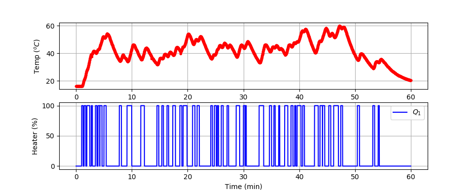
plt.figure(figsize=(10,7)) ax = plt.subplot(2,1,1) ax.grid() plt.plot(tm/60.0,T1,'r.',label=r'$T_1$') plt.ylabel(r'Temp ($^oC$)') ax = plt.subplot(2,1,2) ax.grid() plt.plot(tm/60.0,Q1,'b-',label=r'$Q_1$') plt.ylabel(r'Heater (%)') plt.xlabel('Time (min)') plt.legend() plt.savefig('tclab_data.png') plt.show() (:sourceend:) (:divend:)

Select and scale (0-1) the features of the data such as temperature and temperature slope.

Data for Testing

(:toggle hide tclab_test button show="Generate New TCLab Data for Testing (10 min)":) (:div id=tclab_test:)

Develop a classifier to predict when the TCLab heater is on. Generate labeled data where the heater is either on at 100% output or at 0% output for periods between 10 and 30 seconds or use sample On/Off data. Select and scale (0-1) the features of the data such as temperature and temperature slope.

Q1[190:206] = 100.0

(:toggle hide tclab_data button show="Generate New TCLab Data for Training, Testing, or Validation":)

Q1[260:291] = 100.0

Classification with machine learning is through supervised (labeled outcomes), unsupervised (unlabeled outcomes), or with semi-supervised (some labeled outcomes) methods. From the many methods for classification the best one depends on the problem objectives, data characteristics, and data availability. Below is a complete compilation of the source code for supervised and unsupervised learning methods.

(:title Classification with Machine Learning:)

classifier.predict(digits.data[n:n+1])[0]

(:toggle hide number button show="Number Classification Source (Complete)":)

1. Create Support Vector Classifier

1. Learn / Fit

1. Predict

print(classifier.predict(digits.data[n:n+1])[0])

(:toggle hide number button show="Classify Number Images Source":) (:div id=number:) (:source lang=python:) from sklearn import datasets, svm, metrics from sklearn.model_selection import train_test_split import matplotlib.pyplot as plt import numpy as np

1. The digits dataset

digits = datasets.load_digits() n_samples = len(digits.images) data = digits.images.reshape((n_samples, -1))

1. Create support vector classifier

classifier = svm.SVC(gamma=0.001)

1. Split into train and test subsets (50% each)

X_train, X_test, y_train, y_test = train_test_split(

    data, digits.target, test_size=0.5, shuffle=False)

1. Learn the digits on the first half of the digits

classifier.fit(X_train, y_train)

1. test on second half of data

n = np.random.randint(int(n_samples/2),n_samples) plt.imshow(digits.images[n], cmap=plt.cm.gray_r, interpolation='nearest') print('Predicted: ' + str(classifier.predict(digits.data[n:n+1])[0])) (:sourceend:) (:divend:)

sc = SpectralClustering(n_clusters=2,eigen_solver='arpack', affinity='nearest_neighbors')

1. 0 = Linear, 1 = Quadratic, 2 = Inner Target
2. 3 = Moons, 4 = Concentric Circles, 5 = Distinct Clusters

    y = np.array([False if X[i,0]**2>=X[i,1]+(np.random.rand()-0.5)                  *mixing else True for i in range(n)])

dtree = DecisionTreeClassifier(max_depth=10,random_state=101,max_features=None, min_samples_leaf=5)

rfm = RandomForestClassifier(n_estimators=70,oob_score=True,n_jobs=1, random_state=101,max_features=None,min_samples_leaf=3)

clf = MLPClassifier(solver='lbfgs',alpha=1e-5,max_iter=200, activation='relu',hidden_layer_sizes=(10,30,10), random_state=1, shuffle=True)

sc = SpectralClustering(n_clusters=2,eigen_solver='arpack', affinity='nearest_neighbors')

Classify Number Images

sgd = SGDClassifier(loss='modified_huber',shuffle=True,random_state=101)

dtree = DecisionTreeClassifier(max_depth=10,random_state=101, max_features=None,min_samples_leaf=5)

rfm = RandomForestClassifier(n_estimators=70,oob_score=True,n_jobs=1, random_state=101,max_features=None,min_samples_leaf=3)

clf = MLPClassifier(solver='lbfgs',alpha=1e-5,max_iter=200, activation='relu',hidden_layer_sizes=(10,30,10), random_state=1, shuffle=True)

(:title Classification Machine Learning:) (:keywords classification, segregation, decision, artificial intelligence, machine learning, tutorial, scikit-learn, gekko:) (:description Supervised and unsupervised machine learning methods make a classification decision based on feature inputs.:)

Classification is the problem of identifying which set of categories based on observation features. The decision is based on a training set of data containing observations where category membership is known (supervised learning) or where category membership is unknown (unsupervised learning). A basic example is to determine the number from pixelated images in a built-in sklearn dataset. The script predicts 0-9 from the following images with a Support Vector Classifier.

(:source lang=python:) from sklearn import datasets, svm, metrics from sklearn.model_selection import train_test_split import matplotlib.pyplot as plt import numpy as np

1. The digits dataset

digits = datasets.load_digits() n_samples = len(digits.images) data = digits.images.reshape((n_samples, -1))

1. Create support vector classifier

classifier = svm.SVC(gamma=0.001)

1. Split into train and test subsets (50% each)

X_train, X_test, y_train, y_test = train_test_split(

    data, digits.target, test_size=0.5, shuffle=False)

1. Learn the digits on the first half of the digits

classifier.fit(X_train, y_train)

1. test on second half of data

n = np.random.randint(int(n_samples/2),n_samples) plt.imshow(digits.images[n], cmap=plt.cm.gray_r, interpolation='nearest') print('Predicted: ' + str(classifier.predict(digits.data[n:n+1])[0])) (:sourceend:)

In this case, the 8x8 (64) pixels are the input features to the classifier. The output of the classifier is a number from 0 to 9. The classifier is trained on 898 images and tested on the other 50% of the data. This is an example of supervised learning where the data is labeled with the correct number. An unsupervised learning method would not have the number labels on the training set. An unsupervised learning method creates categories instead of using labels.

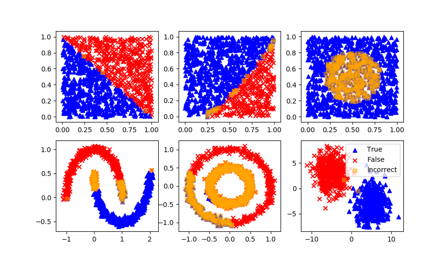
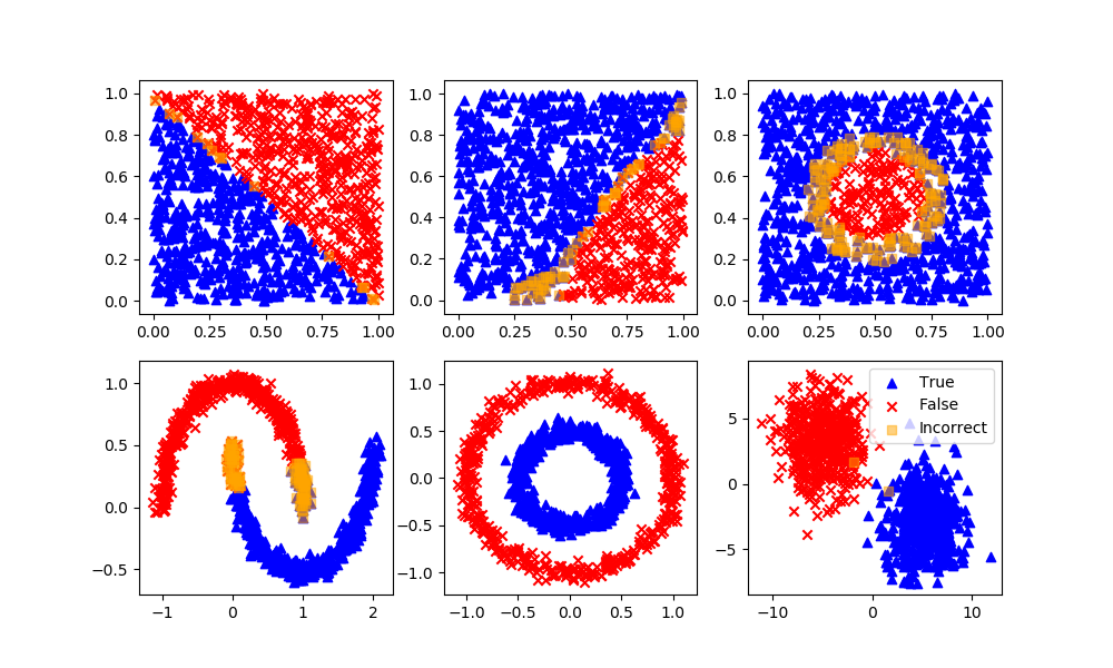
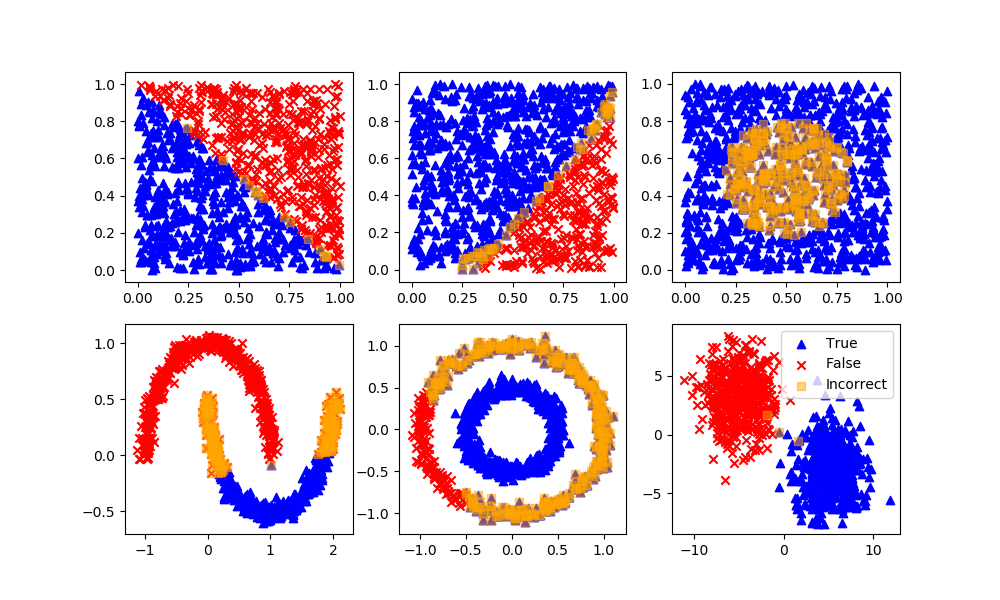
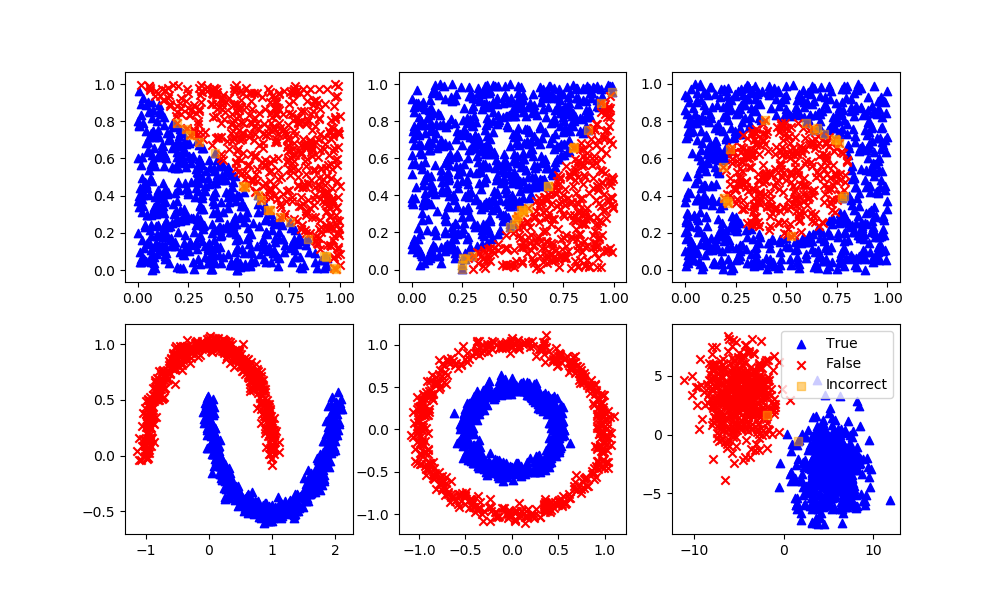
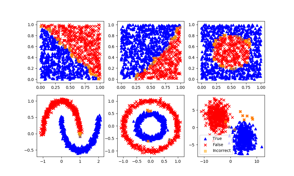
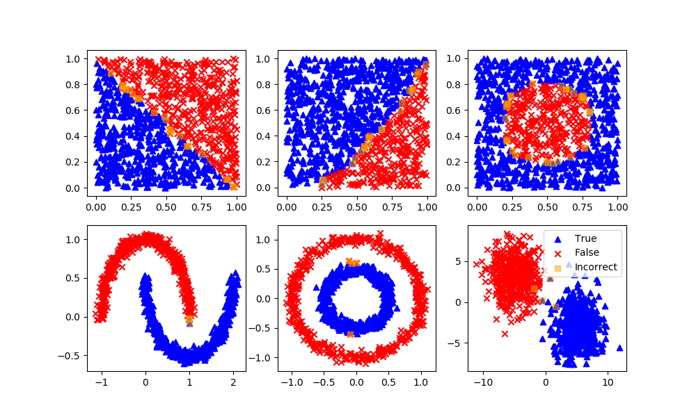
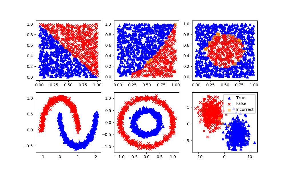
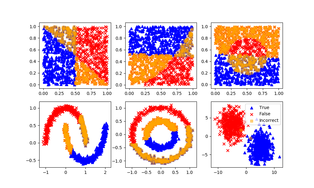
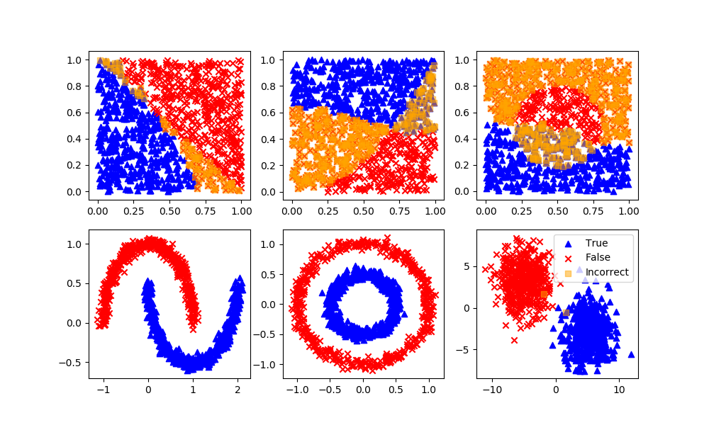
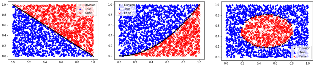
The first step in classification is to curate the data. This typically involves enumeratation, scaling, outlier detection, and splitting the data into training, test, and an optional validation set. One way to learn about classification methods is through concrete examples where the results are visualized as 2D data. The homogeneous data needs data labels (True/False) because there is no segregation of the data that is required for unsupervised learning methods.

Homogeneous Population: 0=Linear, 1=Quadratic, 2=Target

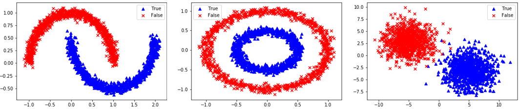
Segregated Clusters: 3=Moons, 4=Concentric Circles, 5=Distinct Clusters

(:toggle hide gen button show="Generate Data":) (:div id=gen:) (:source lang=python:) select_option = 3

data_options = ['linear','quadratic','target','moons','circles','blobs'] option = data_options[select_option] n = 2000 # number of data points

X = np.random.random((n,2)) mixing = 0.0 # add random mixing element to data xplot = np.linspace(0,1,100)

if option=='linear':

    y = np.array([False if (X[i,0]+X[i,1])>=(1.0+mixing/2-np.random.rand()*mixing)                     else True                   for i in range(n)])
    yplot = 1-xplot

elif option=='quadratic':

    y = np.array([False if X[i,0]**2>=X[i,1]+(np.random.rand()-0.5)*mixing                     else True                   for i in range(n)])
    yplot = xplot**2

elif option=='target':

    y = np.array([False if (X[i,0]-0.5)**2+(X[i,1]-0.5)**2<=0.1 +(np.random.rand()-0.5)*0.2*mixing                     else True                   for i in range(n)])
    j = False
    yplot = np.empty(100)
    for i,x in enumerate(xplot):
        r = 0.1-(x-0.5)**2
        if r<=0:
            yplot[i] = np.nan
        else:
            j = not j # plot both sides of circle
            yplot[i] = (2*j-1)*np.sqrt(r)+0.5

elif option=='moons':

    X, y = datasets.make_moons(n_samples=n,noise=0.05)
    yplot = xplot*0.0

elif option=='circles':

    X, y = datasets.make_circles(n_samples=n,noise=0.05,factor=0.5)
    yplot = xplot*0.0

elif option=='blobs':

    X, y = datasets.make_blobs(n_samples=n,centers=-5,3],[5,-3?,cluster_std=2.0)
    yplot = xplot*0.0

plt.scatter(X[y>0.5,0],X[y>0.5,1],color='blue',marker='^',label='True') plt.scatter(X[y<0.5,0],X[y<0.5,1],color='red',marker='x',label='False') if option not in ['moons','circles','blobs']:

    plt.plot(xplot,yplot,'k.',label='Division')

plt.legend()

1. Split into train and test subsets (50% each)

XA, XB, yA, yB = train_test_split(X, y, test_size=0.5, shuffle=False)

1. Plot regression results

def assess(P):

    plt.figure()
    plt.scatter(XB[P==1,0],XB[P==1,1],marker='^',color='blue',label='True')
    plt.scatter(XB[P==0,0],XB[P==0,1],marker='x',color='red',label='False')
    plt.scatter(XB[P!=yB,0],XB[P!=yB,1],marker='s',color='orange',alpha=0.5,label='Incorrect')
    if option not in ['moons','circles','blobs']:
        plt.plot(xplot,yplot,'k.',label='Division')
    plt.legend()

(:sourceend:) (:divend:)

For each of the supervised and unsupervised machine learning methods, the strengths and weaknesses are detailed. The more popular methods are reviewed although there are many new methods that are developed each year. The same principles of training, testing, and deployment are common to most learning methods.

Classification with Supervised Learning

Logistic Regression

Definition: Logistic regression is a machine learning algorithm for classification. In this algorithm, the probabilities describing the possible outcomes of a single trial are modelled using a logistic function.

Advantages: Logistic regression is designed for this purpose (classification), and is most useful for understanding the influence of several independent variables on a single outcome variable.

Disadvantages: Works only when the predicted variable is binary, assumes all predictors are independent of each other, and assumes data is free of missing values.

(:source lang=python:) from sklearn.linear_model import LogisticRegression lr = LogisticRegression(solver='lbfgs') lr.fit(XA,yA) yP = lr.predict(XB) assess(yP) (:sourceend:)

Naïve Bayes

Definition: Naive Bayes algorithm based on Bayes’ theorem with the assumption of independence between every pair of features. Naive Bayes classifiers work well in many real-world situations such as document classification and spam filtering.

Advantages: This algorithm requires a small amount of training data to estimate the necessary parameters. Naive Bayes classifiers are extremely fast compared to more sophisticated methods.

Disadvantages: Naive Bayes is is known to be a bad estimator.

(:source lang=python:) from sklearn.naive_bayes import GaussianNB nb = GaussianNB() nb.fit(XA,yA) yP = nb.predict(XB) assess(yP) (:sourceend:)

Stochastic Gradient Descent

Definition: Stochastic gradient descent is a simple and very efficient approach to fit linear models. It is particularly useful when the number of samples is very large. It supports different loss functions and penalties for classification.

Advantages: Efficiency and ease of implementation.

Disadvantages: Requires a number of hyper-parameters and it is sensitive to feature scaling.

(:source lang=python:) from sklearn.linear_model import SGDClassifier sgd = SGDClassifier(loss='modified_huber', shuffle=True,random_state=101) sgd.fit(XA,yA) yP = sgd.predict(XB) assess(yP) (:sourceend:)

K-Nearest Neighbours

Definition: Neighbours based classification is a type of lazy learning as it does not attempt to construct a general internal model, but simply stores instances of the training data. Classification is computed from a simple majority vote of the k nearest neighbours of each point.

Advantages: This algorithm is simple to implement, robust to noisy training data, and effective if training data is large.

Disadvantages: Need to determine the value of K and the computation cost is high as it needs to computer the distance of each instance to all the training samples. A feedback loop can be added to determine the number of neighbors.

(:source lang=python:) from sklearn.neighbors import KNeighborsClassifier knn = KNeighborsClassifier(n_neighbors=5) knn.fit(XA,yA) yP = knn.predict(XB) assess(yP) (:sourceend:)

Decision Tree

Definition: Given a data of attributes together with its classes, a decision tree produces a sequence of rules that can be used to classify the data.

Advantages: Decision Tree is simple to understand and visualise, requires little data preparation, and can handle both numerical and categorical data.

Disadvantages: Decision tree can create complex trees that do not generalise well, and decision trees can be unstable because small variations in the data might result in a completely different tree being generated.

(:source lang=python:) from sklearn.tree import DecisionTreeClassifier dtree = DecisionTreeClassifier(max_depth=10,random_state=101,max_features=None,min_samples_leaf=5) dtree.fit(XA,yA) yP = dtree.predict(XB) assess(yP) (:sourceend:)

Random Forest

Definition: Random forest classifier is a meta-estimator that fits a number of decision trees on various sub-samples of datasets and uses average to improve the predictive accuracy of the model and controls over-fitting. The sub-sample size is always the same as the original input sample size but the samples are drawn with replacement.

Advantages: Reduction in over-fitting and random forest classifier is more accurate than decision trees in most cases.

Disadvantages: Slow real time prediction, difficult to implement, and complex algorithm.

(:source lang=python:) from sklearn.ensemble import RandomForestClassifier rfm = RandomForestClassifier(n_estimators=70,oob_score=True,n_jobs=1,random_state=101,max_features=None,min_samples_leaf=3) rfm.fit(XA,yA) yP = rfm.predict(XB) assess(yP) (:sourceend:)

Support Vector Classifier

Definition: Support vector machine is a representation of the training data as points in space separated into categories by a clear gap that is as wide as possible. New examples are then mapped into that same space and predicted to belong to a category based on which side of the gap they fall.

Advantages: Effective in high dimensional spaces and uses a subset of training points in the decision function so it is also memory efficient.

Disadvantages: The algorithm does not directly provide probability estimates, these are calculated using an expensive five-fold cross-validation.

(:source lang=python:) from sklearn.svm import SVC svm = SVC(gamma='scale', C=1.0, random_state=101) svm.fit(XA,yA) yP = svm.predict(XB) assess(yP) (:sourceend:)

Deep Learning Neural Network

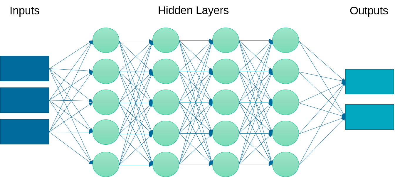
Definition: A neural network is a set of neurons (activation functions) in layers that are processed sequentially to relate an input to an output. This example implements a multi-layer perceptron (MLP) algorithm that trains using Backpropagation.

Advantages: Effective in nonlinear spaces where the structure of the relationship is not linear. No prior knowledge or specialized equation structure is defined although there are different network architectures that may lead to a better result.

Disadvantages: Neural networks do not extrapolate well outside of the training domain. They may also require longer to train by adjusting the parameter weights to minimize a loss (objective) function. It is also more challenging to explain the outcome of the training and changes in initialization or number of epochs (iterations) may lead to different results. Too many epochs may lead to overfitting, especially if there are excess parameters beyond the minimum needed to capture the input to output relationship.

(:source lang=python:) from sklearn.neural_network import MLPClassifier clf = MLPClassifier(solver='lbfgs',alpha=1e-5,max_iter=200,activation='relu', hidden_layer_sizes=(10,30,10), random_state=1, shuffle=True) clf.fit(XA,yA) yP = clf.predict(XB) assess(yP) (:sourceend:)

Classification with Unsupervised Learning

K-Means Clustering

Definition: Specify how many possible clusters (or K) there are in the dataset. The algorithm then iteratively moves the K-centers and selects the datapoints that are closest to that centroid in the cluster.

Advantages: The most common and simplest clustering algorithm.

Disadvantages: Must specify the number of clusters although this can typically be determined by increasing the number of clusters until the objective function does not change significantly.

(:source lang=python:) from sklearn.cluster import KMeans km = KMeans(n_clusters=2) km.fit(XA) yP = km.predict(XB)

1. Arbitrary labels with unsupervised clustering may need to be reversed

if len(XB[yP!=yB]) > n/4: yP = 1 - yP assess(yP) (:sourceend:)

Gaussian Mixture Model

Definition: Data points that exist at the boundary of clusters may simply have similar probabilities of being on either clusters. A mixture model predicts a probability instead of a hard classification such as K-Means clustering.

Advantages: Incorporates uncertainty into the solution.

Disadvantages: Uncertainty may not be desirable for some applications. This method is not as common as the K-Means method for clustering.

(:source lang=python:) from sklearn.mixture import GaussianMixture gmm = GaussianMixture(n_components=2) gmm.fit(XA) yP = gmm.predict_proba(XB) # produces probabilities

1. Arbitrary labels with unsupervised clustering may need to be reversed

if len(XB[np.round(yP[:,0])!=yB]) > n/4: yP = 1 - yP assess(np.round(yP[:,0])) (:sourceend:)

Spectral Clustering

Definition: Spectral clustering is known as segmentation-based object categorization. It is a technique with roots in graph theory, where identify communities of nodes in a graph are based on the edges connecting them. The method is flexible and allows clustering of non graph data as well. It uses information from the eigenvalues of special matrices built from the graph or the data set.

Advantages: Flexible approach for finding clusters when data doesn’t meet the requirements of other common algorithms.

Disadvantages: For large-sized graphs, the second eigenvalue of the (normalized) graph Laplacian matrix is often ill-conditioned, leading to slow convergence of iterative eigenvalue solvers. Spectral clustering is computationally expensive unless the graph is sparse and the similarity matrix can be efficiently constructed.

(:source lang=python:) from sklearn.cluster import SpectralClustering sc = SpectralClustering(n_clusters=2,eigen_solver='arpack',affinity='nearest_neighbors') yP = sc.fit_predict(XB) # No separation between fit and predict calls

                        # Need to fit and predict on same dataset

1. Arbitrary labels with unsupervised clustering may need to be reversed

if len(XB[yP!=yB]) > n/4: yP = 1 - yP assess(yP) (:sourceend:)

Summary

Below is a complete compilation of the source code for supervised and unsupervised learning methods. A Google Colab link to the Classification Jupyter Notebook is also available.

(:toggle hide all_source button show="All Source Code":) (:div id=all_source:) (:source lang=python:) from sklearn import datasets, svm, metrics from sklearn.model_selection import train_test_split import matplotlib.pyplot as plt import numpy as np

1. The digits dataset

digits = datasets.load_digits()

1. Flatten the image to apply classifier

n_samples = len(digits.images) data = digits.images.reshape((n_samples, -1))

1. Create support vector classifier

classifier = svm.SVC(gamma=0.001)

1. Split into train and test subsets (50% each)

X_train, X_test, y_train, y_test = train_test_split(

    data, digits.target, test_size=0.5, shuffle=False)

1. Learn the digits on the first half of the digits

classifier.fit(X_train, y_train) n_samples/2

1. test on second half of data

n = np.random.randint(int(n_samples/2),n_samples) plt.imshow(digits.images[n], cmap=plt.cm.gray_r, interpolation='nearest') print('Predicted: ' + str(classifier.predict(digits.data[n:n+1])[0]))

1. Select Option by Number
2. 0 = Linear, 1 = Quadratic, 2 = Inner Target, 3 = Moons, 4 = Concentric Circles, 5 = Distinct Clusters

select_option = 5

1. generate data

data_options = ['linear','quadratic','target','moons','circles','blobs'] option = data_options[select_option]

1. number of data points

n = 2000 X = np.random.random((n,2)) mixing = 0.0 # add random mixing element to data xplot = np.linspace(0,1,100)

if option=='linear':

    y = np.array([False if (X[i,0]+X[i,1])>=(1.0+mixing/2-np.random.rand()*mixing) else True for i in range(n)])
    yplot = 1-xplot

elif option=='quadratic':

    y = np.array([False if X[i,0]**2>=X[i,1]+(np.random.rand()-0.5)*mixing else True for i in range(n)])
    yplot = xplot**2

elif option=='target':

    y = np.array([False if (X[i,0]-0.5)**2+(X[i,1]-0.5)**2<=0.1 +(np.random.rand()-0.5)*0.2*mixing else True for i in range(n)])
    j = False
    yplot = np.empty(100)
    for i,x in enumerate(xplot):
        r = 0.1-(x-0.5)**2
        if r<=0:
            yplot[i] = np.nan
        else:
            j = not j # plot both sides of circle
            yplot[i] = (2*j-1)*np.sqrt(r)+0.5

elif option=='moons':

    X, y = datasets.make_moons(n_samples=n,noise=0.05)
    yplot = xplot*0.0

elif option=='circles':

    X, y = datasets.make_circles(n_samples=n,noise=0.05,factor=0.5)
    yplot = xplot*0.0

elif option=='blobs':

    X, y = datasets.make_blobs(n_samples=n,centers=-5,3],[5,-3?,cluster_std=2.0)
    yplot = xplot*0.0

plt.scatter(X[y>0.5,0],X[y>0.5,1],color='blue',marker='^',label='True') plt.scatter(X[y<0.5,0],X[y<0.5,1],color='red',marker='x',label='False') if option not in ['moons','circles','blobs']:

    plt.plot(xplot,yplot,'k.',label='Division')

plt.legend() plt.savefig(str(select_option)+'.png')

1. Split into train and test subsets (50% each)

XA, XB, yA, yB = train_test_split(X, y, test_size=0.5, shuffle=False)

1. Plot regression results

def assess(P):

    plt.figure()
    plt.scatter(XB[P==1,0],XB[P==1,1],marker='^',color='blue',label='True')
    plt.scatter(XB[P==0,0],XB[P==0,1],marker='x',color='red',label='False')
    plt.scatter(XB[P!=yB,0],XB[P!=yB,1],marker='s',color='orange',alpha=0.5,label='Incorrect')
    if option not in ['moons','circles','blobs']:
        plt.plot(xplot,yplot,'k.',label='Division')
    plt.legend()

1. Supervised Classification
2. Logistic Regression

from sklearn.linear_model import LogisticRegression lr = LogisticRegression(solver='lbfgs') lr.fit(XA,yA) yP = lr.predict(XB) assess(yP)

1. Naïve Bayes

from sklearn.naive_bayes import GaussianNB nb = GaussianNB() nb.fit(XA,yA) yP = nb.predict(XB) assess(yP)

1. Stochastic Gradient Descent

from sklearn.linear_model import SGDClassifier sgd = SGDClassifier(loss='modified_huber', shuffle=True,random_state=101) sgd.fit(XA,yA) yP = sgd.predict(XB) assess(yP)

1. K-Nearest Neighbours

from sklearn.neighbors import KNeighborsClassifier knn = KNeighborsClassifier(n_neighbors=5) knn.fit(XA,yA) yP = knn.predict(XB) assess(yP)

1. Decision Tree

from sklearn.tree import DecisionTreeClassifier dtree = DecisionTreeClassifier(max_depth=10,random_state=101,max_features=None,min_samples_leaf=5) dtree.fit(XA,yA) yP = dtree.predict(XB) assess(yP)

1. Random Forest

from sklearn.ensemble import RandomForestClassifier rfm = RandomForestClassifier(n_estimators=70,oob_score=True,n_jobs=1,random_state=101,max_features=None,min_samples_leaf=3) rfm.fit(XA,yA) yP = rfm.predict(XB) assess(yP)

1. Support Vector Classifier

from sklearn.svm import SVC svm = SVC(gamma='scale', C=1.0, random_state=101) svm.fit(XA,yA) yP = svm.predict(XB) assess(yP)

1. Neural Network

from sklearn.neural_network import MLPClassifier clf = MLPClassifier(solver='lbfgs',alpha=1e-5,max_iter=200,activation='relu',hidden_layer_sizes=(10,30,10), random_state=1, shuffle=True) clf.fit(XA,yA) yP = clf.predict(XB) assess(yP)

1. Unsupervised Classification
2. K-Means Clustering

from sklearn.cluster import KMeans km = KMeans(n_clusters=2) km.fit(XA) yP = km.predict(XB)

1. Arbitrary labels with unsupervised clustering may need to be reversed

if len(XB[yP!=yB]) > n/4: yP = 1 - yP assess(yP)

1. Gaussian Mixture Model

from sklearn.mixture import GaussianMixture gmm = GaussianMixture(n_components=2) gmm.fit(XA) yP = gmm.predict_proba(XB) # produces probabilities

1. Arbitrary labels with unsupervised clustering may need to be reversed

if len(XB[np.round(yP[:,0])!=yB]) > n/4: yP = 1 - yP assess(np.round(yP[:,0]))

1. Spectral Clustering

from sklearn.cluster import SpectralClustering sc = SpectralClustering(n_clusters=2,eigen_solver='arpack',affinity='nearest_neighbors') yP = sc.fit_predict(XB) # No separation between fit and predict calls, need to fit and predict on same dataset

1. Arbitrary labels with unsupervised clustering may need to be reversed

if len(XB[yP!=yB]) > n/4: yP = 1 - yP assess(yP)

plt.show() (:sourceend:) (:divend:)

Exercise

Develop a classifier to predict when the TCLab heater is on. Generate labeled data where the heater is either on at 100% output or at 0% output for periods between 10 and 30 seconds or use sample On/Off data. Select and scale (0-1) the features of the data such as temperature and temperature slope.

(:toggle hide tclab_data button show="Generate New TCLab Data for Training and Validation":) (:div id=tclab_data:)

(:source lang=python:)

1. generate new data

import numpy as np import matplotlib.pyplot as plt import pandas as pd import tclab import time

n = 600 # Number of second time points (10 min) tm = np.linspace(0,n,n+1) # Time values lab = tclab.TCLab() T1 = [lab.T1] T2 = [lab.T2] Q1 = np.zeros(n+1) Q2 = np.zeros(n+1) Q1[20:41] = 100.0 Q1[60:91] = 100.0 Q1[150:181] = 100.0 Q1[190:191] = 100.0 Q1[220:251] = 100.0 Q1[300:316] = 100.0 Q1[340:351] = 100.0 Q1[400:431] = 100.0 Q1[500:521] = 100.0 Q1[540:571] = 100.0 for i in range(n):

    lab.Q1(Q1[i])
    lab.Q2(Q2[i])
    time.sleep(1)
    print(Q1[i],lab.T1)
    T1.append(lab.T1)
    T2.append(lab.T2)

lab.close()

1. Save data file

data = np.vstack((tm,Q1,Q2,T1,T2)).T np.savetxt('tclab_data.csv',data,delimiter=',', header='Time,Q1,Q2,T1,T2',comments='')

1. Create Figure

plt.figure(figsize=(10,7)) ax = plt.subplot(2,1,1) ax.grid() plt.plot(tm/60.0,T1,'r.',label=r'$T_1$') plt.ylabel(r'Temp ($^oC$)') ax = plt.subplot(2,1,2) ax.grid() plt.plot(tm/60.0,Q1,'b-',label=r'$Q_1$') plt.ylabel(r'Heater (%)') plt.xlabel('Time (min)') plt.legend() plt.savefig('tclab_data.png') plt.show() (:sourceend:) (:divend:)

Use the measured temperature and heater values to create a classifier that predicts when the heater is on or off. Validate the classifier with a new data set.

(:toggle hide TCLab_classifier button show="Show TCLab Classifier Solution":) (:div id=TCLab_classifier:)

TCLab Classifier Solution

Coming soon... (:divend:)