Dynamic Estimation Objectives

The dynamic estimation objective function is a mathematical statement that is minimized or maximized to find a best solution among all possible feasible solutions. The form of this objective function is critical to give desirable solutions for model predictions but also for other applications that use the output of a dynamic estimation application. Two common objective functions are shown below as squared error and l₁-norm forms¹.

Squared Error Objective

The squared error objective is the most common form, used extensively in the literature. It is also the basis for the derivation of the Kalman filter and other well known estimators.

$$\min_{x,y,p} \Phi = \left(y_x-y\right)^T W_x \left(y_x-y\right) + \left(y-\hat y\right)^T W_m \left(y-\hat y\right) + \Delta p^T W_{\Delta p} \Delta p$$

$$\mathrm{subject\;\;to}$$

$$0 = f\left(\frac{dx}{dt},x,y,p\right)$$

$$0 \le g\left(\frac{dx}{dt},x,y,p\right)$$

l₁-norm Objective

The l₁-norm objective is like an absolute value objective but also includes a dead-band to reject measurement error and stabilize the parameter estimates.

$$\min_{x,y,p} \Phi = w_x^T \left(e_U+e_L\right) + w_m^T \left(c_U+c_L\right) + w_{\Delta p}^T \left(\Delta p_U+\Delta p_L\right)$$

$$\mathrm{subject\;\;to}$$

$$0 = f\left(\frac{dx}{dt},x,y,p\right)$$

$$0 \le g\left(\frac{dx}{dt},x,y,p\right)$$

$$e_U \ge y - y_x - \frac{db}{2}$$

$$e_L \ge y_x - y - \frac{db}{2}$$

$$c_U \ge y - \hat y$$

$$c_L \ge \hat y - y$$

$$\Delta p_U \ge p_i - p_{i-1}$$

$$\Delta p_L \ge p_{i-1} - p_i$$

$$e_U, e_L, c_U, c_L, \Delta p_U, \Delta p_L \ge 0$$

The l₁-norm objective is like an absolute value of the error but posed in a way to have continuous first and second derivatives. The addition of slack variables enables an efficient formulation (only linear constraints) that is also convex (local optimum is the global optimum). A unique aspect of the following l₁-norm objective is the addition of a dead-band or region around the measurements where there is no penalty. It is only when the model predictions are outside of this dead-band that the optimizer makes changes to the parameters to correct the model.

Nomenclature

There are many symbols used in the definition of the different objective function forms. Below is a nomenclature table that gives a description of each variable and the role in the objective expression.

$$\Phi=\mathrm{Objective\,Function}$$

$$y_x=\mathrm{measurements}$$

$$y=\mathrm{model\,predictions}$$

$$\hat y=\mathrm{prior\,model\,values}$$

$$w_x, W_x=\mathrm{measurement\,deviation\,penalty\,(WMEAS)}$$

$$w_m, W_m=\mathrm{prior\,prediction\,deviation\,penalty\,(WMODEL)}$$

$$w_{\Delta p},W_{\Delta p}=\mathrm{parameter\,movement\,penalty\,(DCOST)}$$

$$db=\mathrm{dead-band\,for\,noise\,rejection}$$

$$x,y,p=\mathrm{states,\,outputs,\,parameters}$$

$$\Delta p=\mathrm{parameter\,change}$$

$$f,g=\mathrm{equality\,and\,inequality\,constraints}$$

$$e_U,e_L=\mathrm{upper\,and\,lower\,error\,outside\,dead-band}$$

$$c_U,c_L=\mathrm{upper\,and\,lower\,deviation\,from\,prior\,model\,prediction}$$

$$\Delta p_U,\Delta p_L=\mathrm{upper\,and\,lower\,parameter\,change}$$

The following example problem is a demonstration of the two different objective forms and some of the configuration to achieve optimal estimator performance.

Motion Estimation from GPS Position (1D Example)

Exercise

Objective: Estimate parameters of a highly nonlinear system. Use an initialization strategy to find a suitable approximation for the parameter estimation. Create a MATLAB or Python script to simulate and display the results. Estimated Time: 2 hours

The spread of HIV in a patient is approximated with balance equations on (H)ealthy, (I)nfected, and (V)irus population counts². Additional information on the HIV model is at the Process Dynamic and Control Course.

 Initial Conditions
 H = healthy cells = 1,000,000
 I = infected cells = 0
 V = virus = 100
 LV = log virus = 2

 Equations
 dH/dt = kr1 - kr2 H - kr3 H V
 dI/dt = kr3 H V - kr4 I
 dV/dt = -kr3 H V - kr5 V + kr6 I
 LV = log10(V)

There are six parameters (kr_1..6) in the model that provide the rates of cell death, infection spread, virus replication, and other processes that determine the spread of HIV in the body.

 Parameters
 kr1 = new healthy cells
 kr2 = death rate of healthy cells
 kr3 = healthy cells converting to infected cells
 kr4 = death rate of infected cells
 kr5 = death rate of virus
 kr6 = production of virus by infected cells

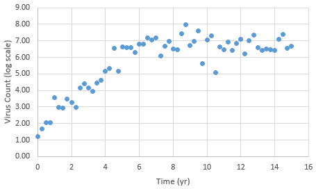
The following data is provided from a virus count over the course of 15 years. Note that the virus count information is reported in log scale.

HIV Data and Model Files

With guess values for parameters (kr_1..6), approximately match the laboratory data for this patient as an initial solution. Use this initial solution to compute an optimal solution with dynamic estimation. Adjust parameters kr_1..6 to match the virus count data. Start with different kr values to verify that the solution is not just locally optimal but also globally optimal.

Solution

HIV Estimation in MATLAB and Python

References

1. Safdarnejad, S.M., Hedengren, J.D., Lewis, N.R., Haseltine, E., Initialization Strategies for Optimization of Dynamic Systems, Computers and Chemical Engineering, 2015, Vol. 78, pp. 39-50, DOI: 10.1016/j.compchemeng.2015.04.016. Article
2. Hedengren, J. D. and Asgharzadeh Shishavan, R., Powell, K.M., and Edgar, T.F., Nonlinear Modeling, Estimation and Predictive Control in APMonitor, Computers and Chemical Engineering, Volume 70, pg. 133–148, 2014. Article
3. Nowak, M. and May, R. M. Virus dynamics: mathematical principles of immunology and virology: mathematical principles of immunology and virology. Oxford university press, 2000.
4. Lewis, N.R., Hedengren, J.D., Haseltine, E.L., Hybrid Dynamic Optimization Methods for Systems Biology with Efficient Sensitivities, Special Issue on Algorithms and Applications in Dynamic Optimization, Processes, 2015, 3(3), 701-729; doi:10.3390/pr3030701. Article