Mixed Integer Optimal Control
Main.DiscreteVariables History
Hide minor edits - Show changes to markup
(:html:) <iframe width="560" height="315" src="https://www.youtube.com/embed/RPKPjqdiX1c" frameborder="0" allowfullscreen></iframe> (:htmlend:)
(:title Dynamic Control with Discrete Variables:)
(:title Mixed Integer Optimal Control:)

(:html:) <iframe width="560" height="315" src="//www.youtube.com/embed/XhqteZIydT0?rel=0" frameborder="0" allowfullscreen></iframe> (:htmlend:)
Exercise 2
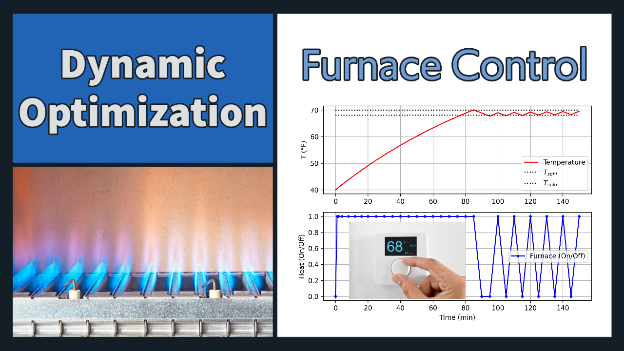
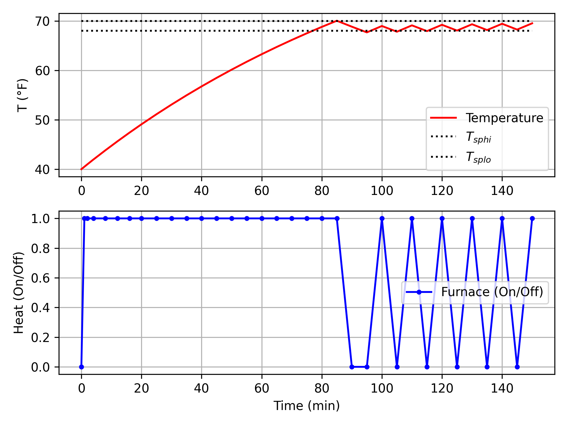
Design a thermostat for a home that has a furnace with On/Off control. The home is initially unheated in 40 degF weather. When the heater is turned on, the temperature in the home reaches 63% of the steady state value in 120 minutes, starting from 40 degF. If left on indefinitely, the home would eventually reach 100 degF. Optimize the heater response for the first 2 1/2 hours starting from a cold home at 40 degF. The target range for the home is between 68 and 70 degF.
Solution
(:toggle hide python button show="Show Python GEKKO Source":) (:div id=python:) (:source lang=python:) from gekko import GEKKO import matplotlib.pyplot as plt
m = GEKKO() # create GEKKO model m.time = [0,1,2,4,8,12,16,20,25,30,35,40,45,50, 55,60,65,70,75,80,85,90,95,100,105,110, 115,120,125,130,135,140,145,150]
- change solver options
m.solver_options = ['minlp_gap_tol 1.0e-2', 'minlp_maximum_iterations 10000', 'minlp_max_iter_with_int_sol 5000'] m.options.SOLVER = 1 m.options.IMODE = 6
- parameters
Kp = 60 taup = 120 T0 = 40
- create heater binary variable
u = m.MV(integer=True,lb=0,ub=1) u.dcost = 0.1 u.status = 1
- controlled variable (temperature)
T = m.CV(value=T0) T.SPHI = 68 T.SPLO = 70 T.STATUS = 1 T.TR_INIT = 0
- first order equation
m.Equation(taup * T.dt() == -(T-T0) + Kp * u)
m.solve() # solve MILP
- plot solution
plt.subplot(2,1,1) plt.plot(m.time,T,'r-',label='Temperature') plt.plot([0,m.time[-1]],[T.SPHI,T.SPHI],'k:',label=r'$T_{sphi}$') plt.plot([0,m.time[-1]],[T.SPLO,T.SPLO],'k:',label=r'$T_{splo}$') plt.ylabel('T (degF)') plt.legend() plt.subplot(2,1,2) plt.plot(m.time,u,'b.-',label='Furnace (On/Off)') plt.ylabel('Heat (On/Off)') plt.xlabel('Time (min)') plt.legend() plt.show() (:sourceend:) (:divend:)
(:html:) <iframe width="560" height="315" src="https://www.youtube.com/embed/2XC6mpop_j4" frameborder="0" allowfullscreen></iframe> (:htmlend:)
Exercise 3
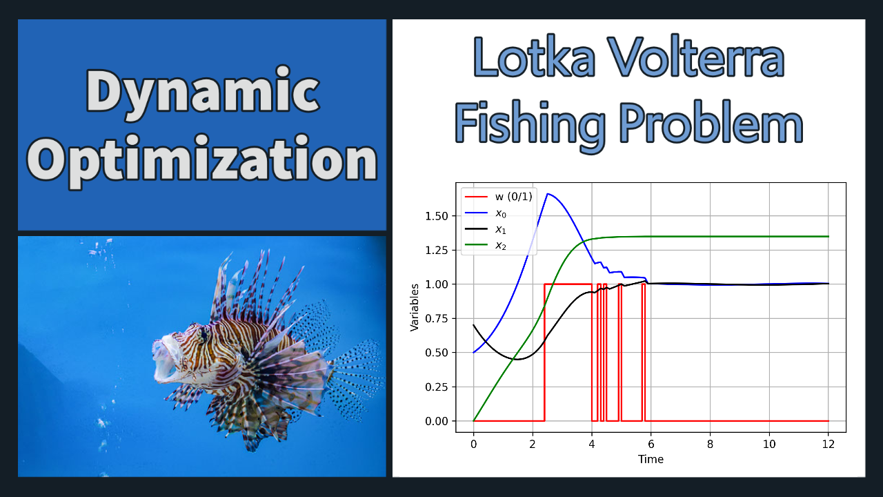
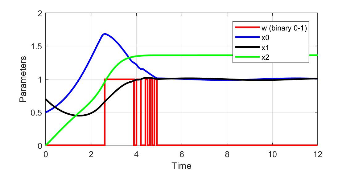
An example problem for Mixed Integer Optimal Control is the Lotka Volterra fishing problem. It finds an fishing strategy over a 12 year horizon to equilibrate the predator-prey fish to a sustainable steady-state value. The Lotka Volterra equations for a predator-prey system have an additional equation to introduce fishing by man and with constants `c_0=0.4` and `c_1=0.2`.
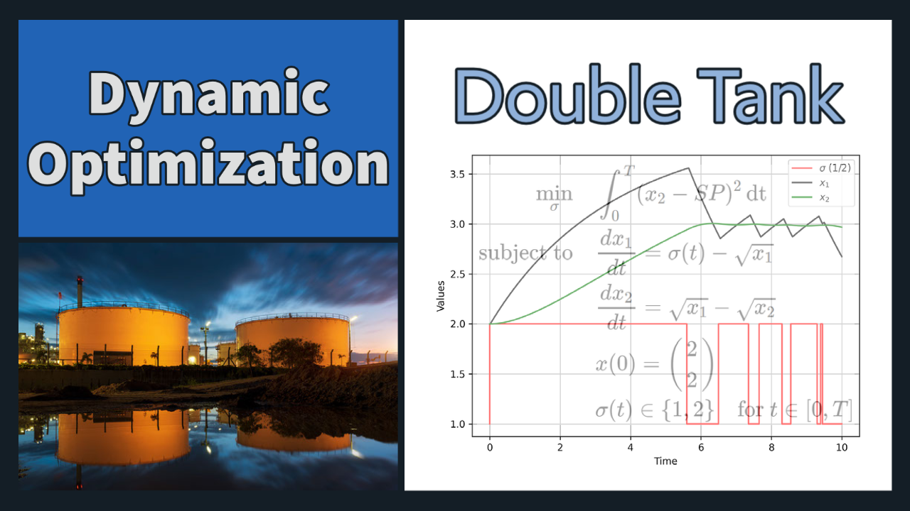
$$\min_{x,w} x_2 \left( t_f \right)$$
$$\mathrm{s.t.} \quad \frac{dx_0}{dt} = x_0 - x_0 x_1 - c_0 x_0 w$$ $$\quad \quad \frac{dx_1}{dt} = -x_1 + x_0 x_1 - c_1 x_1 w$$ $$\quad \quad \frac{dx_2}{dt} = \left(x_0-1\right)^2 + \left(x_1-1\right)^2$$ $$\quad \quad x(0) = (0.5,0.7,0)^T$$ $$\quad \quad w(t) \in {{0,1}}$$
The optimal solution has a final objective of 1.344.
(:toggle hide solution2 button show="Show Python GEKKO Solution":) (:div id=solution2:) (:source lang=python:) import numpy as np import matplotlib.pyplot as plt from gekko import GEKKO
m = GEKKO() # create GEKKO model
- Add 0.01 as first step
- 0,0.01,0.1,0.2,0.3,...11.9,12.0)
m.time = np.insert(np.linspace(0,12,121),1,0.01)
- change solver options
m.solver_options = ['minlp_gap_tol 0.001', 'minlp_maximum_iterations 10000', 'minlp_max_iter_with_int_sol 100', 'minlp_branch_method 1', 'minlp_integer_tol 0.001', 'minlp_integer_leaves 0', 'minlp_maximum_iterations 200']
c0 = 0.4 c1 = 0.2
last = m.Param(np.zeros(122)) last.value[-1] = 1
x0 = m.Var(value=0.5,lb=0) x1 = m.Var(value=0.7,lb=0) x2 = m.Var(value=0.0,lb=0) w = m.MV(value=0,lb=0,ub=1,integer=True) w.STATUS = 1
m.Obj(last*x2)
m.Equations([x0.dt() == x0 - x0*x1 - c0*x0*w, x1.dt() == - x1 + x0*x1 - c1*x1*w, x2.dt() == (x0-1)**2 + (x1-1)**2])
m.options.IMODE = 6 m.options.NODES = 3 m.options.SOLVER = 1 m.options.MV_TYPE = 0 m.solve()
plt.figure(1) plt.step(m.time,w.value,'r-',label='w (0/1)') plt.plot(m.time,x0.value,'b-',label=r'$x_0$') plt.plot(m.time,x1.value,'k-',label=r'$x_1$') plt.plot(m.time,x2.value,'g-',label=r'$x_2$') plt.xlabel('Time') plt.ylabel('Variables') plt.legend(loc='best') plt.show() (:sourceend:) (:divend:)
Integer Variables
Integer Variables in Gekko
Integer variables are defined in Python Gekko with the integer=True option when declaring the variable. A Special Ordered Set is also possible to define discrete options that are not necessarily integers.
(:source lang=python:) x = m.Var(lb=0,ub=1,integer=True) # binary variable (0-1) y = m.Var(lb=0,ub=8,integer=True) # integer variable (0,1,..,7,8) z = m.sos1([0.5,1.25,2.5]) # discrete variable (0.5,1.25,2.5) (:sourceend:)
Additional mixed-integer tutorials in APMonitor and Gekko.
Integer Variables in APMonitor
(:toggle hide solution button show="Show APM Python Solution":) (:div id=solution:) (:source lang=python:) import numpy as np import matplotlib.pyplot as plt from APMonitor.apm import *
- write model
model = '''
apopt MINLP solver options (see apopt.com)
File apopt.opt
 minlp_maximum_iterations 1000     ! minlp iterations
 minlp_max_iter_with_int_sol 50    ! minlp iterations if integer solution is found
 minlp_as_nlp 0                    ! treat minlp as nlp
 nlp_maximum_iterations 200        ! nlp sub-problem max iterations
 minlp_branch_method 1             ! 1 = depth first, 2 = breadth first
 minlp_gap_tol 0.001               ! covergence tolerance
 minlp_integer_tol 0.001           ! maximum deviation from whole number to be considered an integer
 minlp_integer_leaves 0            ! create soft (1) integer leaves or hard (2) integer leaves with branching
End File
Constants
  c0 = 0.4
  c1 = 0.2
Parameters
last
Variables
  x0 = 0.5 , >= 0
  x1 = 0.7 , >= 0
  x2 = 0.0 , >= 0
  int_w = 0 , >= 0 , <= 1
Intermediates
w = int_w
Equations
  minimize last * x2

  $x0 = x0 - x0*x1 - c0*x0*w
  $x1 = - x1 + x0*x1 - c1*x1*w
  $x2 = (x0-1)^2 + (x1-1)^2
''' fid = open('lotka_volterra.apm','w') fid.write(model) fid.close()
- write data file
time = np.linspace(0,12,121) time = np.insert(time, 1, 0.01) last = np.zeros(122) last[-1] = 1.0 data = np.vstack((time,last)) np.savetxt('data.csv',data.T,delimiter=',',header='time,last',comments='')
- specify server and application name
s = 'https://byu.apmonitor.com'
- s = 'https://127.0.0.1/' # for local APMonitor server
a = 'lotka'
apm(s,a,'clear all') apm_load(s,a,'lotka_volterra.apm') csv_load(s,a,'data.csv')
apm_option(s,a,'nlc.imode',6) # Nonlinear control / dynamic optimization apm_option(s,a,'nlc.nodes',3)
apm_info(s,a,'MV','int_w') # M or MV = Manipulated variable - independent variable over time horizon apm_option(s,a,'int_w.status',1) # Status: 1=ON, 0=OFF apm_option(s,a,'int_w.mv_type',0) # MV Type = Zero Order Hold
apm_option(s,a,'nlc.solver',1) # 1 = APOPT
- solve
output = apm(s,a,'solve') print(output)
- retrieve solution
y = apm_sol(s,a)
plt.figure(1) plt.step(y['time'],y['int_w'],'r-',label='w (0/1)') plt.plot(y['time'],y['x0'],'b-',label=r'$x_0$') plt.plot(y['time'],y['x1'],'k-',label=r'$x_1$') plt.plot(y['time'],y['x2'],'g-',label=r'$x_2$') plt.xlabel('Time') plt.ylabel('Variables') plt.legend(loc='best') plt.show() (:sourceend:) (:divend:)
An example problem for Mixed Integer Optimal Control is the Lotka Volterra fishing problem. It finds an fishing strategy over a 12 year horizon to equilibrate the predator as prey fish to a minimum steady state value. The Lotka Volterra equations for a predator-prey system have an additional equation to introduce fishing by man and with constants `c_0=0.4` and `c_1=0.2`.
An example problem for Mixed Integer Optimal Control is the Lotka Volterra fishing problem. It finds an fishing strategy over a 12 year horizon to equilibrate the predator-prey fish to a sustainable steady-state value. The Lotka Volterra equations for a predator-prey system have an additional equation to introduce fishing by man and with constants `c_0=0.4` and `c_1=0.2`.
plt.xlabel('Time') plt.ylabel('Variables') plt.legend(loc='best') plt.show() (:sourceend:) (:divend:)
(:toggle hide solution2 button show="Show Python GEKKO Solution":) (:div id=solution2:) (:source lang=python:) import numpy as np import matplotlib.pyplot as plt from gekko import GEKKO
m = GEKKO() # create GEKKO model
- Add 0.01 as first step
- 0,0.01,0.1,0.2,0.3,...11.9,12.0)
m.time = np.insert(np.linspace(0,12,121),1,0.01)
- change solver options
m.solver_options = ['minlp_gap_tol 0.001', 'minlp_maximum_iterations 10000', 'minlp_max_iter_with_int_sol 100', 'minlp_branch_method 1', 'minlp_integer_tol 0.001', 'minlp_integer_leaves 0', 'minlp_maximum_iterations 200']
c0 = 0.4 c1 = 0.2
last = m.Param(np.zeros(122)) last.value[-1] = 1
x0 = m.Var(value=0.5,lb=0) x1 = m.Var(value=0.7,lb=0) x2 = m.Var(value=0.0,lb=0) w = m.MV(value=0,lb=0,ub=1,integer=True) w.STATUS = 1
m.Obj(last*x2)
m.Equations([x0.dt() == x0 - x0*x1 - c0*x0*w, x1.dt() == - x1 + x0*x1 - c1*x1*w, x2.dt() == (x0-1)**2 + (x1-1)**2])
m.options.IMODE = 6 m.options.NODES = 3 m.options.SOLVER = 1 m.options.MV_TYPE = 0 m.solve()
plt.figure(1) plt.step(m.time,w.value,'r-',label='w (0/1)') plt.plot(m.time,x0.value,'b-',label=r'$x_0$') plt.plot(m.time,x1.value,'k-',label=r'$x_1$') plt.plot(m.time,x2.value,'g-',label=r'$x_2$')
(:toggle hide solution button show="Show Python Solution":)
(:toggle hide solution button show="Show APM Python Solution":)
- retrieve apm.py from
- https://raw.githubusercontent.com/APMonitor/apm_python/master/apm.py
- or
- https://apmonitor.com/wiki/index.php/Main/PythonApp
from apm import *
- alternative pip install with 'pip install APMonitor'
- from APMonitor.apm import *
- local APMonitor servers are available for Windows or Linux
- https://apmonitor.com/wiki/index.php/Main/APMonitorServer
- with clients in Python, MATLAB, and Julia
from APMonitor.apm import *
Solution
Solve integer problem with Python GEKKO. Set integer=True to switch the variable from continuous to integer form. The APOPT solver is required to solve problem with integer variables but other solvers such as IPOPT can provide a relaxed solution where the integer conditions are not enforced.
Solution
The integer problem is solved with Python GEKKO. The option integer=True is used to switch the variable from continuous to integer form. The APOPT solver is required to solve problem with integer variables but other solvers such as IPOPT can provide a relaxed solution where the integer conditions are not enforced.
Solution
(:toggle hide python button show="Show Python GEKKO Source":) (:div id=python:) (:source lang=python:) from gekko import GEKKO import matplotlib.pyplot as plt
m = GEKKO() # create GEKKO model m.time = [0,1,2,4,8,12,16,20,25,30,35,40,45,50, 55,60,65,70,75,80,85,90,95,100,105,110, 115,120,125,130,135,140,145,150]
- change solver options
m.solver_options = ['minlp_gap_tol 1.0e-2', 'minlp_maximum_iterations 10000', 'minlp_max_iter_with_int_sol 5000'] m.options.SOLVER = 1 m.options.IMODE = 6
- parameters
Kp = 60 taup = 120 T0 = 40
- create heater binary variable
u = m.MV(integer=True,lb=0,ub=1) u.dcost = 0.1 u.status = 1
- controlled variable (temperature)
T = m.CV(value=T0) T.SPHI = 68 T.SPLO = 70 T.STATUS = 1 T.TR_INIT = 0
- first order equation
m.Equation(taup * T.dt() == -(T-T0) + Kp * u)
m.solve() # solve MILP
- plot solution
plt.subplot(2,1,1) plt.plot(m.time,T,'r-',label='Temperature') plt.plot([0,m.time[-1]],[T.SPHI,T.SPHI],'k:',label=r'$T_{sphi}$') plt.plot([0,m.time[-1]],[T.SPLO,T.SPLO],'k:',label=r'$T_{splo}$') plt.ylabel('T (degF)') plt.legend() plt.subplot(2,1,2) plt.plot(m.time,u,'b.-',label='Furnace (On/Off)') plt.ylabel('Heat (On/Off)') plt.xlabel('Time (min)') plt.legend() plt.show() (:sourceend:) (:divend:)
Solve integer problem with Python GEKKO. Set integer=True to switch the variable from continuous to integer form. The APOPT solver is required to solve problem with integer variables but other solvers such as IPOPT can provide a relaxed solution where the integer conditions are not enforced.
(:source lang=python:) from gekko import GEKKO m = GEKKO() # create GEKKO model
- create integer variables
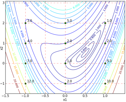
x1 = m.Var(integer=True,lb=-1,ub=1) x2 = m.Var(integer=True,lb=-1,ub=2) m.Obj(4*x1**2-4*x2*x1**2+x2**2+x1**2-x1+1) m.options.SOLVER = 1 # APOPT solver m.solve() print('x1: ' + str(x1.value[0])) print('x2: ' + str(x2.value[0])) (:sourceend:)
(:source lang=python:)
(:sourceend:)
$$\min_{x,w} x_2\left(t_f\right$$
$$\min_{x,w} x_2 \left( t_f \right)$$
$$\quad \quad \frac{dx_0}{dt} = \left(x_0-1\right)^2 + \left(x_1-1\right)^2$$
$$\quad \quad \frac{dx_2}{dt} = \left(x_0-1\right)^2 + \left(x_1-1\right)^2$$
$$\quad \quad x(t) \in {0,1}$$
$$\quad \quad w(t) \in {{0,1}}$$
The optimal solution has a final objective of 1.344.
(:toggle hide solution button show="Show Python Solution":) (:div id=solution:) import numpy as np import matplotlib.pyplot as plt
- retrieve apm.py from
- https://raw.githubusercontent.com/APMonitor/apm_python/master/apm.py
- or
- https://apmonitor.com/wiki/index.php/Main/PythonApp
from apm import *
- alternative pip install with 'pip install APMonitor'
- from APMonitor.apm import *
- local APMonitor servers are available for Windows or Linux
- https://apmonitor.com/wiki/index.php/Main/APMonitorServer
- with clients in Python, MATLAB, and Julia
- write model
model = '''
apopt MINLP solver options (see apopt.com)
File apopt.opt
 minlp_maximum_iterations 1000     ! minlp iterations
 minlp_max_iter_with_int_sol 50    ! minlp iterations if integer solution is found
 minlp_as_nlp 0                    ! treat minlp as nlp
 nlp_maximum_iterations 200        ! nlp sub-problem max iterations
 minlp_branch_method 1             ! 1 = depth first, 2 = breadth first
 minlp_gap_tol 0.001               ! covergence tolerance
 minlp_integer_tol 0.001           ! maximum deviation from whole number to be considered an integer
 minlp_integer_leaves 0            ! create soft (1) integer leaves or hard (2) integer leaves with branching
End File
Constants
  c0 = 0.4
  c1 = 0.2
Parameters
last
Variables
  x0 = 0.5 , >= 0
  x1 = 0.7 , >= 0
  x2 = 0.0 , >= 0
  int_w = 0 , >= 0 , <= 1
Intermediates
w = int_w
Equations
  minimize last * x2

  $x0 = x0 - x0*x1 - c0*x0*w
  $x1 = - x1 + x0*x1 - c1*x1*w
  $x2 = (x0-1)^2 + (x1-1)^2
''' fid = open('lotka_volterra.apm','w') fid.write(model) fid.close()
- write data file
time = np.linspace(0,12,121) time = np.insert(time, 1, 0.01) last = np.zeros(122) last[-1] = 1.0 data = np.vstack((time,last)) np.savetxt('data.csv',data.T,delimiter=',',header='time,last',comments='')
- specify server and application name
s = 'https://byu.apmonitor.com'
- s = 'https://127.0.0.1/' # for local APMonitor server
a = 'lotka'
apm(s,a,'clear all') apm_load(s,a,'lotka_volterra.apm') csv_load(s,a,'data.csv')
apm_option(s,a,'nlc.imode',6) # Nonlinear control / dynamic optimization apm_option(s,a,'nlc.nodes',3)
apm_info(s,a,'MV','int_w') # M or MV = Manipulated variable - independent variable over time horizon apm_option(s,a,'int_w.status',1) # Status: 1=ON, 0=OFF apm_option(s,a,'int_w.mv_type',0) # MV Type = Zero Order Hold
apm_option(s,a,'nlc.solver',1) # 1 = APOPT
- solve
output = apm(s,a,'solve') print(output)
- retrieve solution
y = apm_sol(s,a)
plt.figure(1) plt.step(y['time'],y['int_w'],'r-',label='w (0/1)') plt.plot(y['time'],y['x0'],'b-',label=r'$x_0$') plt.plot(y['time'],y['x1'],'k-',label=r'$x_1$') plt.plot(y['time'],y['x2'],'g-',label=r'$x_2$') plt.xlabel('Time') plt.ylabel('Variables') plt.legend(loc='best') plt.show() (:divend:)
Exercise 3
An example problem for Mixed Integer Optimal Control is the Lotka Volterra fishing problem. It finds an fishing strategy over a 12 year horizon to equilibrate the predator as prey fish to a minimum steady state value. The Lotka Volterra equations for a predator-prey system have an additional equation to introduce fishing by man and with constants `c_0=0.4` and `c_1=0.2`.
$$\min_{x,w} x_2\left(t_f\right$$
$$\mathrm{s.t.} \quad \frac{dx_0}{dt} = x_0 - x_0 x_1 - c_0 x_0 w$$ $$\quad \quad \frac{dx_1}{dt} = -x_1 + x_0 x_1 - c_1 x_1 w$$ $$\quad \quad \frac{dx_0}{dt} = \left(x_0-1\right)^2 + \left(x_1-1\right)^2$$ $$\quad \quad x(0) = (0.5,0.7,0)^T$$ $$\quad \quad x(t) \in {0,1}$$
- Mixed Integer Optimal Control Problems
- Mixed Integer Optimal Control Problems (mintOC)
- Mixed Integer Optimal Control Problems
- CMU-IBM Cyber-Infrastructure for MINLP
(:htmlend:)
Integer Variables
Integer or binary variables are defined in the APMonitor Modeling Language by appending a variable name with int. An binary decision variable is an integer variable with bounds between 0 and 1.
 ! Binary decision variable (0 or 1)
 Variables
   int_b >=0 <=1
The range of upper and lower bounds can be increased or decreased to any range to create a more general integer variable.
 ! Integer decision variable (-5 to 10)
 Variables
   int_v >=-5 <=10
Nonlinear programming solvers (such as IPOPT) may not return an integer solution because they are designed for continuous variables. Mixed Integer Nonlinear Programming solvers (such as APOPT) are equipped to solve for binary or integer variables. Select the appropriate solver option to either find an initial solution without integer variables or an integer solution. It is sometimes desirable to find a non-integer solution first because of the often significant reduction in computation time without the integer variables.
(:html:) <iframe width="560" height="315" src="https://www.youtube.com/embed/RPKPjqdiX1c" frameborder="0" allowfullscreen></iframe> (:htmlend:)
(:html:) <iframe width="560" height="315" src="https://www.youtube.com/embed/2XC6mpop_j4" frameborder="0" allowfullscreen></iframe> (:htmlend:)
Exercise
Exercise 1
Exercise 2
Design a thermostat for a home that has a furnace with On/Off control. The home is initially unheated in 40 degF weather. When the heater is turned on, the temperature in the home reaches 63% of the steady state value in 120 minutes, starting from 40 degF. If left on indefinitely, the home would eventually reach 100 degF. Optimize the heater response for the first 2 1/2 hours starting from a cold home at 40 degF. The target range for the home is between 68 and 70 degF.
Objective: Solve a discrete optimization problem with the branch and bound technique. Estimated time: 2 hours.
Objective: Solve a discrete optimization problem with the branch and bound technique. Estimated time: 1 hour.
Discrete decision variables are those that have only certain levels or quantities that are acceptable at an optimal solution. Examples of discrete variables are binary (e.g. off/on or 0/1), integer (e.g. 4,5,6,7), or general discrete values that are not integer (e.g. 1/4 cm, 1/2 cm, 1 cm).
One often encounters problems in which manipulated variables or adjustable parameters must be selected from among a set of discrete values. Examples of discrete variables include ON/OFF state, selection of different feed lines, and other variables that are naturally integers. Many dynamic optimization problems are discrete in nature.
At first glance it might seem solving a discrete variable problem would be easier than a continuous problem. After all, for a variable within a given range, a set of discrete values within the range is finite whereas the number of continuous values is infinite. When searching for an optimum, it seems it would be easier to search from a finite set rather than from an infinite set.
This is not the case, however. Solving discrete problems is harder than continuous problems. This is because of the combinatorial explosion that occurs in all but the smallest problems. For example if we have two variables which can each take 10 values, we have 10*10 = 100 possibilities. If we have 10 variables that can each take 10 values, we have 10^10 possibilities. Even with the fastest computer, it would take a long time to evaluate all of these.
Discrete decision variables are those that have only certain levels or quantities that are acceptable at an optimal solution. Examples of discrete variables are binary (e.g. off/on or 0/1), integer (e.g. 4,5,6,7), or general discrete values that are not integer (e.g. 1/4 cm, 1/2 cm, 1 cm).
Exercise
Objective: Solve a discrete optimization problem with the branch and bound technique. Estimated time: 2 hours.
Solution
(:html:) <iframe width="560" height="315" src="//www.youtube.com/embed/XhqteZIydT0?rel=0" frameborder="0" allowfullscreen></iframe> (:htmlend:)
(:title Dynamic Control with Discrete Variables:) (:keywords dynamic control, model predictive control, integer, binary, discrete:) (:description Model predictive control may require binary (On/Off), integer (select number of pumps), or other discrete decision variables:)
Discrete decision variables are those that have only certain levels or quantities that are acceptable at an optimal solution. Examples of discrete variables are binary (e.g. off/on or 0/1), integer (e.g. 4,5,6,7), or general discrete values that are not integer (e.g. 1/4 cm, 1/2 cm, 1 cm).