Many Single Input, Single Output (SISO) dynamic systems can be represented empirically with a First Order Plus Dead Time (FOPDT) model. Model identification involves fitting parameters in a dynamic continuous or discrete form of the FOPDT model. The unknown parameters for this system include the time constant (`\tau`), gain (K), and sometimes dead-time (`\theta`).
$$\tau \frac{dx}{dt} = -x + K \, u\left(t-\theta\right)$$
Model/Process Mismatch
The time constant and gain may be incorrect because of system nonlinearity, bad data, or process drift over time. If the model is used in a model predictive controller, a model gain that is lower than the actual process gain may cause controller oscillation and instability. A model gain that is higher than the actual process may cause sluggish control. Likewise, a model response (time constant) that is slow (higher time constant) than the actual process time constant tends to cause controller instability. On the other hand, a model response (time constant) that is fast (lower time constant) than the actual process tends to cause sluggish controller response. This is illustrated by the following objective function plot that shows model predictive control performance with model mismatch to the process.
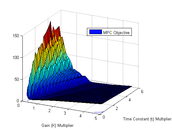
The combination of a low gain and high time constant leads to the highest objective function (poor performance and instability). On the other hand, a high gain and low time constant lead to sluggish control but the controller is able to asymptotically drive the process to the correct set point.
Exercise
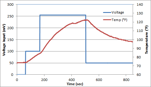
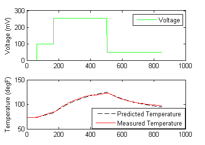
For this exercise, you can assume that the dead-time (`\theta`) is zero and estimate only the time constant (`\tau`) and gain (K). The following data set was generated in class from a voltage input (u) that changed the temperature (x) of a thermistor from the Arduino Lab.

Fit the dynamic data to a first order linear system by estimating `\tau` (time constant) and K (gain). Determine the 95% and 99% confidence intervals for the parameters (see F-test video tutorial).
Excel Solution
The dynamic model can be written in discrete form by specifying that the voltage is constant between sampling intervals. The discrete form of the equation accounts for non-zero initial conditions in temperature (x0) and voltage (u0). In this case, the voltage does start at zero, but this is not required.
$$x_k = \left(x_{k-1}-x_0\right) e^{-\Delta t/\tau} + \left(u_{k-1}-u_0\right)K\left(1-e^{-\Delta t/\tau}\right) + x_0$$
In this equation, the subscripts denote the sampling intervals that are collected at a time interval of delta time = tk-tk-1. The above equation and the data are put into an Excel worksheet. The difference between the measured and predicted values are minimized to obtain the optimal parameters K (gain) and `\tau` (time constant).
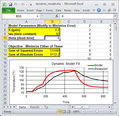
The spreadsheet is currently showing non-optimal values. To obtain the optimal values, use Excel Solver available from the Data toolbar. If the solver option does not appear, it can be added with the Add-In manager.

MATLAB and Python Solutions
An alternative approach to the sum of squared errors is to minimize an l1-norm error to find the optimal values of K (gain) and `\tau` (time constant).
The MATLAB and Python plots produce trends that show the optimal solution with an l1-norm objective function.
The nonlinear confidence interval is shown by producing a contour plot of the SSE objective function with variations in the two parameters. The optimal solution is shown at the center of the plot and the objective function becomes worse (higher) away from the optimal solution.
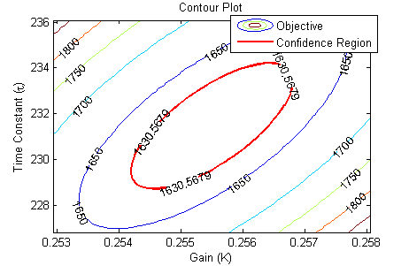
The confidence interval is determined with an F-test that specifies an upper limit to the deviation from the optimal solution
$$\frac{SSE(\theta)-SSE(\theta^*)}{SSE(\theta^*)}\le \frac{p}{n-p} F\left(\alpha,p,n-p\right)$$
with p=2 (number of parameters), n=851 (number of measurements), `\theta`=[K,`\tau`] (parameters), `\theta^*` as the optimal parameters, SSE as the sum of squared errors, and the F statistic that has 3 arguments (alpha=confidence level, degrees of freedom 1, and degrees of freedom 2). For many problems, this creates a multi-dimensional nonlinear confidence region. In the case of 2 parameters, the nonlinear confidence region is a 2-dimensional space.
Solution (GEKKO Python)
import numpy as np
import pandas as pd
import matplotlib.pyplot as plt
# load data and parse into columns
url = 'http://apmonitor.com/do/uploads/Main/tclab_siso_data.txt'
data = pd.read_csv(url)
t = data['time']
u = data['voltage']
y = data['temperature']
# generate time-series model
m = GEKKO()
# system identification
na = 2 # output coefficients
nb = 2 # input coefficients
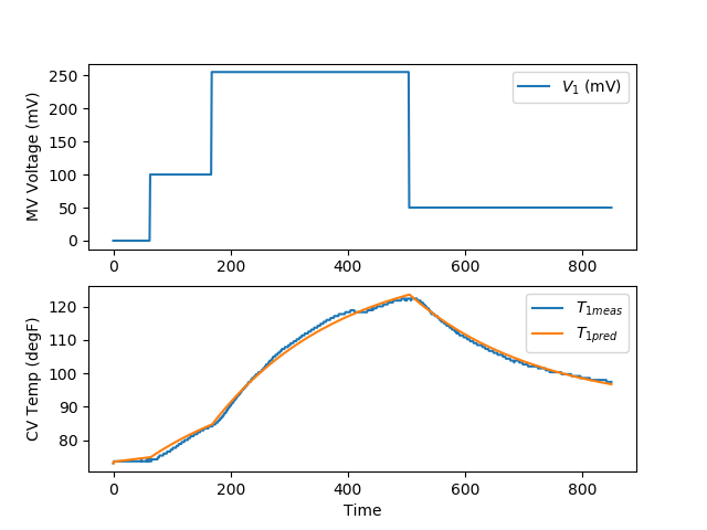
yp,p,K = m.sysid(t,u,y,na,nb,pred='meas')
plt.figure()
plt.subplot(2,1,1)
plt.plot(t,u)
plt.legend([r'$V_1$ (mV)'])
plt.ylabel('MV Voltage (mV)')
plt.subplot(2,1,2)
plt.plot(t,y)
plt.plot(t,yp)
plt.legend([r'$T_{1meas}$',r'$T_{1pred}$'])
plt.ylabel('CV Temp (degF)')
plt.xlabel('Time')
plt.savefig('sysid.png')
plt.show()
import numpy as np
import pandas as pd
import matplotlib.pyplot as plt
# load data and parse into columns
url = 'http://apmonitor.com/do/uploads/Main/tclab_siso_data.txt'
data = pd.read_csv(url)
t = data['time']
u = data['voltage']
y = data['temperature']
# generate time-series model
m = GEKKO()
# system identification
na = 2 # output coefficients
nb = 2 # input coefficients
yp,p,K = m.sysid(t,u,y,na,nb,pred='meas')
plt.figure()
plt.subplot(2,1,1)
plt.plot(t,u)
plt.legend([r'$V_1$ (mV)'])
plt.ylabel('MV Voltage (mV)')
plt.subplot(2,1,2)
plt.plot(t,y)
plt.plot(t,yp)
plt.legend([r'$T_{1meas}$',r'$T_{1pred}$'])
plt.ylabel('CV Temp (degF)')
plt.xlabel('Time')
plt.savefig('sysid.png')
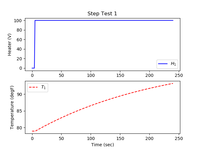
# step test model
yc,uc = m.arx(p)
# steady state initialization
m.options.IMODE = 1
m.solve(disp=False)
# dynamic simulation (step test)
m.time = np.linspace(0,240,241)
m.options.TIME_SHIFT=0
m.options.IMODE = 4
m.solve(disp=False)
# step for first MV (Heater 1)
uc[0].value = np.zeros(len(m.time))
uc[0].value[5:] = 100
m.solve(disp=False)
plt.figure()
plt.subplot(2,1,1)
plt.title('Step Test 1')
plt.plot(m.time,uc[0].value,'b-',label=r'$H_1$')
plt.ylabel('Heater (V)')
plt.legend()
plt.subplot(2,1,2)
plt.plot(m.time,yc[0].value,'r--',label=r'$T_1$')
plt.ylabel('Temperature (degF)')
plt.legend()
plt.xlabel('Time (sec)')
plt.legend()
plt.savefig('step_test.png')
plt.show()