Dynamic Control Objectives
Main.ControllerObjective History
Hide minor edits - Show changes to markup
plt.plot(m.time,p.value,'b-',LineWidth=2,label='MV')
plt.plot(m.time,p.value,'b-',lw=2,label='MV')
plt.plot(m.time,v.value,'r--',LineWidth=2,label='CV')
plt.plot(m.time,v.value,'r--',lw=2,label='CV')
plt.plot(m.time,p.value,'b-',LineWidth=2,label='MV')
plt.plot(m.time,p.value,'b-',lw=2,label='MV')
plt.plot(m.time,v.value,'r--',LineWidth=2,label='CV')
plt.plot(m.time,v.value,'r--',lw=2,label='CV')
plt.plot(m.time,e.value,'r--',LineWidth=2,label='Error')
plt.plot(m.time,e.value,'r--',lw=2,label='Error')
$$y,x,u=\mathrm{outputs\,states\,and\,inputs}$$
$$y,x,u=\mathrm{outputs,\,states,\,and\,inputs}$$
$$\min_{x,y,u} \Phi = \left(y-y_t\right)^T W_t \left(y-y_t\right) + y^T c_y + u^T c_u + \Delta u^T c_{\Delta u} \Delta u$$
$$\min_{x,y,u} \Phi = \left(y-y_t\right)^T W_t \left(y-y_t\right) + y^T w_y + u^T w_u + \Delta u^T W_{\Delta u} \Delta u$$
$$\min_{x,y,u} \Phi = w_{hi}^T e_{hi} + w_{lo}^T e_{lo} + y^T c_y + u^T c_u + w_{\Delta u}^T \left(\Delta u_U+\Delta u_L\right)$$
$$\min_{x,y,u} \Phi = w_{hi}^T e_{hi} + w_{lo}^T e_{lo} + y^T w_y + u^T w_u + w_{\Delta u}^T \left(\Delta u_U+\Delta u_L\right)$$
$$c_{\Delta u}=\mathrm{manipulated\,variable\,movement\,penalty\,(DCOST)}$$
$$W_{\Delta u}, w_{\Delta u}=\mathrm{manipulated\,variable\,movement\,penalty\,(DCOST)}$$
$$w_{u}, w_{y}=\mathrm{weight\,on\,input\,and\,output\,(COST)}$$
$$0 = f\left(\frac{dx}{dt},x,y,p\right)$$
$$0 \le g\left(\frac{dx}{dt},x,y,p\right)$$
$$0 = f\left(\frac{dx}{dt},x,y,u\right)$$
$$0 \le g\left(\frac{dx}{dt},x,y,u\right)$$
$$y_t,y_{t,hi},y_{t,lo}=\mathrm{reference trajectory or range}$$
$$y_t,y_{t,hi},y_{t,lo}=\mathrm{reference\,trajectory\,or\,range}$$
$$\tau_c \frac{dy_{t,hi}}{dt} + y_{t,hi} = sp_{hi}$$
$$\tau_c \frac{dy_{t,lo}}{dt} + y_{t,lo} = sp_{lo}$$
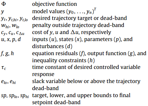
$$\Phi=\mathrm{Objective\,Function}$$
$$y=\mathrm{model\,predictions}$$
$$y_t,y_{t,hi},y_{t,lo}=\mathrm{reference trajectory or range}$$
$$W_t,w_{hi}, w_{lo}=\mathrm{penalty\,outside\,reference\,trajectory\,(WSP,WSPHI,WSPLO)}$$
$$c_{\Delta u}=\mathrm{manipulated\,variable\,movement\,penalty\,(DCOST)}$$
$$y,x,u=\mathrm{outputs\,states\,and\,inputs}$$
$$\Delta u=\mathrm{manipulated\,variable\,change}$$
$$f,g=\mathrm{equality\,and\,inequality\,constraints}$$
$$e_{hi},e_{lo}=\mathrm{upper\,and\,lower\,error\,outside\,dead-band}$$
$$\Delta u_U,\Delta u_L=\mathrm{upper\,and\,lower\,manipulated\,variable\,change}$$
$$\Delta p_U \ge p - \hat p$$
$$\Delta p_L \ge \hat p - p$$
$$e_{hi}, e_{lo}, \Delta p_U, \Delta p_L \ge 0$$
$$\Delta u_U \ge u_i - u_{i-1}$$
$$\Delta u_L \ge u_{i-1} - u_i$$
$$e_{hi}, e_{lo}, \Delta u_U, \Delta u_L \ge 0$$
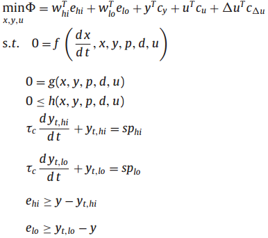
$$\min_{x,y,u} \Phi = w_{hi}^T e_{hi} + w_{lo}^T e_{lo} + y^T c_y + u^T c_u + w_{\Delta u}^T \left(\Delta u_U+\Delta u_L\right)$$
$$\mathrm{subject\;\;to}$$
$$0 = f\left(\frac{dx}{dt},x,y,p\right)$$
$$0 \le g\left(\frac{dx}{dt},x,y,p\right)$$
$$e_{hi} \ge y - y_{t,hi}$$
$$e_{lo} \ge y_{t,lo} - y$$
$$\Delta p_U \ge p - \hat p$$
$$\Delta p_L \ge \hat p - p$$
$$e_{hi}, e_{lo}, \Delta p_U, \Delta p_L \ge 0$$
$$0 = f\left(\frac{d\;x}{d\;t},x,y,u\right)$$
$$0 \le g\left(\frac{d\;x}{d\;t},x,y,u\right)$$
$$\tau_c \frac{d\;y_t}{d\;t} + y_t = sp$$
$$0 = f\left(\frac{dx}{dt},x,y,u\right)$$
$$0 \le g\left(\frac{dx}{dt},x,y,u\right)$$
$$\tau_c \frac{dy_t}{dt} + y_t = sp$$
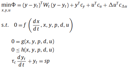
$$\min_{x,y,u} \Phi = \left(y-y_t\right)^T W_t \left(y-y_t\right) + y^T c_y + u^T c_u + \Delta u^T c_{\Delta u} \Delta u$$
$$\mathrm{subject\;\;to}$$
$$0 = f\left(\frac{d\;x}{d\;t},x,y,u\right)$$
$$0 \le g\left(\frac{d\;x}{d\;t},x,y,u\right)$$
$$\tau_c \frac{d\;y_t}{d\;t} + y_t = sp$$

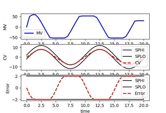
Some applications require a custom reference trajectory that does not fit a standard form. A custom reference trajectory is specified by creating a new error (e) variable that is the difference between the specified trajectory (sinusoidal, sawtooth, random, etc) and the model output. This error is specified as a controlled variable (CV) with an upper and lower dead-band denoted as SPHI and SPLO. The CV can also be a value of zero with a squared error objective (e.SP=0, m.options.CV_TYPE=2) to drive to a target instead of a dead-band range.
e.TR_INIT = 1 #setpoint trajectory
e.TR_INIT = 0 #setpoint trajectory
Reactor Tuning Example
(:html:) <iframe width="560" height="315" src="https://www.youtube.com/embed/qH55ym1g-NM" frameborder="0" allowfullscreen></iframe> (:htmlend:)
Custom Reference Trajectory
(:toggle hide gekko_traj button show="Custom Reference Trajectory with GEKKO":) (:div id=gekko_traj:) (:source lang=python:) import numpy as np from random import random from gekko import GEKKO import matplotlib.pyplot as plt
- initialize GEKKO model
m = GEKKO()
- time
m.time = np.linspace(0,20,41)
- constants
mass = 500
- Parameters
b = m.Param(value=50) K = m.Param(value=0.8)
- Manipulated variable
p = m.MV(value=0, lb=-100, ub=100)
- Reference trajectory
sine = 10*np.sin(m.time/20*4*np.pi) traj = m.Param(value=sine)
- Controlled Variable
v = m.SV(value=0,name='v')
- Error
e = m.CV(value=0,name='e')
- Equations
m.Equation(mass*v.dt() == -v*b + K*b*p) m.Equation(e==v-traj)
m.options.IMODE = 6 # control
- MV tuning
p.STATUS = 1 #allow optimizer to change p.DCOST = 0.1 #smooth out MV p.DMAX = 50 #slow down change of MV
- CV tuning
e.STATUS = 1 #add the CV to the objective m.options.CV_TYPE = 1 #Dead-band db = 2 e.SPHI = db #set point e.SPLO = -db #set point e.TR_INIT = 1 #setpoint trajectory e.TAU = 5 #time constant of setpoint trajectory
- Solve
m.solve()
- get additional solution information
import json with open(m.path+'//results.json') as f:
results = json.load(f)
- Plot solution
plt.figure() plt.subplot(3,1,1) plt.plot(m.time,p.value,'b-',LineWidth=2,label='MV') plt.legend(loc='best') plt.ylabel('MV') plt.subplot(3,1,2) plt.plot(m.time,sine+db,'k-',label='SPHI') plt.plot(m.time,sine-db,'k-',label='SPLO') plt.plot(m.time,v.value,'r--',LineWidth=2,label='CV') plt.legend(loc='best') plt.ylabel('CV') plt.subplot(3,1,3) plt.plot(m.time,results['e.tr_hi'],'k-',label='SPHI') plt.plot(m.time,results['e.tr_lo'],'k-',label='SPLO') plt.plot(m.time,e.value,'r--',LineWidth=2,label='Error') plt.legend(loc='best') plt.ylabel('Error') plt.xlabel('time') plt.show() (:sourceend:) (:divend:)
v = m.CV(value=0)
v = m.CV(value=0,name='v')
plt.plot(m.time,results['v1.tr_lo'],'k-',label='SPHI') plt.plot(m.time,results['v1.tr_hi'],'k-',label='SPLO')
plt.plot(m.time,results['v.tr_lo'],'k-',label='SPHI') plt.plot(m.time,results['v.tr_hi'],'k-',label='SPLO')
(:toggle hide gekko_mpc button show="Model Predictive Control with GEKKO":) (:div id=gekko_mpc:)
(:source lang=python:) import numpy as np from random import random from gekko import GEKKO import matplotlib.pyplot as plt
- initialize GEKKO model
m = GEKKO()
- time
m.time = np.linspace(0,20,41)
- constants
mass = 500
- Parameters
b = m.Param(value=50) K = m.Param(value=0.8)
- Manipulated variable
p = m.MV(value=0, lb=0, ub=100)
- Controlled Variable
v = m.CV(value=0)
- Equations
m.Equation(mass*v.dt() == -v*b + K*b*p)
m.options.IMODE = 6 # control
- MV tuning
p.STATUS = 1 #allow optimizer to change p.DCOST = 0.1 #smooth out MV p.DMAX = 20 #slow down change of MV
- CV tuning
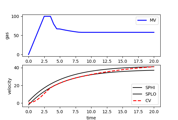
v.STATUS = 1 #add the CV to the objective m.options.CV_TYPE = 1 #Dead-band v.SPHI = 42 #set point v.SPLO = 38 #set point v.TR_INIT = 1 #setpoint trajectory v.TAU = 5 #time constant of setpoint trajectory
- Solve
m.solve()
- get additional solution information
import json with open(m.path+'//results.json') as f:
results = json.load(f)
- Plot solution
plt.figure() plt.subplot(2,1,1) plt.plot(m.time,p.value,'b-',LineWidth=2,label='MV') plt.legend(loc='best') plt.ylabel('gas') plt.subplot(2,1,2) plt.plot(m.time,results['v1.tr_lo'],'k-',label='SPHI') plt.plot(m.time,results['v1.tr_hi'],'k-',label='SPLO') plt.plot(m.time,v.value,'r--',LineWidth=2,label='CV') plt.legend(loc='best') plt.ylabel('velocity') plt.xlabel('time') plt.show() (:sourceend:) (:divend:)
(:html:) <iframe width="560" height="315" src="https://www.youtube.com/embed/dM8gX54jWW4" frameborder="0" allowfullscreen></iframe> (:htmlend:)
The dynamic control objective function is a mathematical statement that is minimized or maximized to find a best solution among all possible feasible solutions for a controller. The form of this objective function is critical to give desirable solutions for driving a system to a desirable state or along a desired trajectory. Common objective statements relate to economic, safety, operability, environmental, or related objectives. Two common objective functions are shown below as squared error and l1-norm forms1.
The dynamic control objective function is a mathematical statement that is minimized or maximized to find a best solution among all possible feasible solutions for a controller. The form of this objective function is critical to give desirable solutions for driving a system to a desirable state or along a desired trajectory. Common objective statements relate to economic, safety, operability, environmental, or related objectives.
Two common objective functions are shown below as squared error and l1-norm forms1.
The l1-norm objective is the absolute value of the difference between the current measured value of the controlled variable and the desired target value. The absolute value operator is
The l1-norm objective is the absolute value of the difference between the current measured value of the controlled variable and the desired target value. The absolute value operator (abs(x)) does not have a continuous first and second derivative at x=0 (see absolute value function alternatives). Slack variables give the same absolute value function but with continuous first and second derivatives.
The squared error objective is the most common form used in the literature. It penalizes deviation of the current measured value of the controlled variable from the desired target value.
The l1-norm objective is the absolute value of the difference between the current measured value of the controlled variable and the desired target value. The absolute value operator is
In formulating an objective function and model equations follow the following tips for improved convergence.
- Rearrange to equation in residual form to:
- Avoid divide by zero
- Minimize use of functions like sqrt, log, exp, etc.
- Have continuous first and second derivatives
- Fit the equation into a linear or quadratic form
- Bounds
- Include variable bounds to exclude infeasible solutions
- Variable bounds to avoid regions of strong nonlinearity
- Caution: watch for infeasible solutions
- Scaling:
- Scale absolute value of variables to 1e-3 to 1e3
- Scale absolute value of equation residuals to 1e-3 to 1e3
- Better that 1st derivative values are closer to 1.0
- Good initial conditions:
- Starting near a solution can improve convergence
- Try multiple initial conditions to verify global solution (non-convex problems)
- Explicitly calculate intermediate values
- Check iteration summary for improved convergence
(:html:) <iframe width="560" height="315" src="https://www.youtube.com/embed/qH55ym1g-NM" frameborder="0" allowfullscreen></iframe> (:htmlend:)
Exercise
Objective: Set up and solve several dynamic optimization benchmark problems2. Create a program to optimize and display the results. Estimated Time (each): 30 minutes
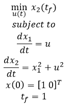
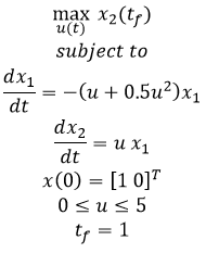
- Example 1a - Nonlinear, unconstrained, minimize final state
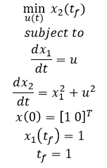
- Example 1b - Nonlinear, unconstrained, minimize final state with terminal constraint
- Example 2 - Nonlinear, constrained, minimize final state
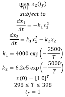
- Example 3 - Tubular reactor with parallel reaction
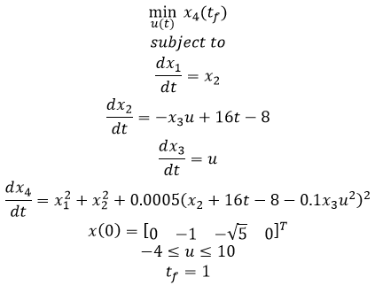
- Example 4 - Batch reactor with consecutive reactions A->B->C
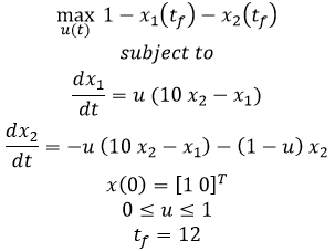
Example 5 - Catalytic reactor with A<->B->C
Solution
(:html:) <iframe width="560" height="315" src="https://www.youtube.com/embed/mmCFF3-6sGg" frameborder="0" allowfullscreen></iframe> (:htmlend:)
- M. Čižniar, M. Fikar, M.A. Latifi: A MATLAB Package for Dynamic Optimisation of Processes, 7th International Scientific – Technical Conference – Process Control 2006, June 13 – 16, 2006, Kouty nad Desnou, Czech Republic. Article
(:html:) <iframe width="560" height="315" src="https://www.youtube.com/embed/mmCFF3-6sGg" frameborder="0" allowfullscreen></iframe> (:htmlend:)
Example 5 - Catalytic plug flow reactor with A->B->C
Example 5 - Catalytic reactor with A<->B->C
Exercise
Objective: Set up and solve several dynamic optimization benchmark problems2. Create a program to optimize and display the results. Estimated Time (each): 30 minutes
- Example 1a - Nonlinear, unconstrained, minimize final state
- Example 1b - Nonlinear, unconstrained, minimize final state with terminal constraint
- Example 2 - Nonlinear, constrained, minimize final state
- Example 3 - Tubular reactor with parallel reaction
- Example 4 - Batch reactor with consecutive reactions A->B->C
Example 5 - Catalytic plug flow reactor with A->B->C
Solution
- M. Čižniar, M. Fikar, M.A. Latifi: A MATLAB Package for Dynamic Optimisation of Processes, 7th International Scientific – Technical Conference – Process Control 2006, June 13 – 16, 2006, Kouty nad Desnou, Czech Republic. Article
Exercise
Objective: Design a model predictive controller with a custom objective function that satisfies a specific problem criterion. Simulate and optimize a pendulum system with an adjustable overhead cart. Estimated time: 3 hours.
A pendulum is described by the following dynamic equations:
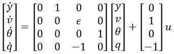
where epsilon is m2/(m1+m2), y is the position of the overhead cart, v is the velocity of the overhead cart, theta is the angle of the pendulum relative to the cart, and q is the rate of angle change2.
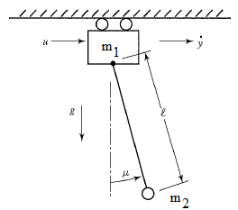
The objective of the controller is to adjust the force on the cart to move the pendulum mass to a new final position. Ensure that initial and final velocities and angles of the pendulum are zero. The position of the pendulum mass is initially at -1 and it is desired to move it to the new position of 0 within 6.2 seconds. Demonstrate controller performance with changes in the pendulum position and that the final pendulum mass remains at the final position without oscillation.
Solution
- Bryson, A.E., Dynamic Optimization, Addison-Wesley, 1999.
where epsilon is m2/(m1+m2), y is the position of the overhead cart, v is the velocity of the overhead cart, theta is the angle of the pendulum relative to the cart, and q is the rate of angle change.
where epsilon is m2/(m1+m2), y is the position of the overhead cart, v is the velocity of the overhead cart, theta is the angle of the pendulum relative to the cart, and q is the rate of angle change2.
- Bryson, A.E., Dynamic Optimization, Addison-Wesley, 1999.
Exercise
Objective: Design a model predictive controller with a custom objective function that satisfies a specific problem criterion. Simulate and optimize a pendulum system with an adjustable overhead cart. Estimated time: 3 hours.
A pendulum is described by the following dynamic equations:
where epsilon is m2/(m1+m2), y is the position of the overhead cart, v is the velocity of the overhead cart, theta is the angle of the pendulum relative to the cart, and q is the rate of angle change.
The objective of the controller is to adjust the force on the cart to move the pendulum mass to a new final position. Ensure that initial and final velocities and angles of the pendulum are zero. The position of the pendulum mass is initially at -1 and it is desired to move it to the new position of 0 within 6.2 seconds. Demonstrate controller performance with changes in the pendulum position and that the final pendulum mass remains at the final position without oscillation.
Solution
- Hedengren, J. D. and Asgharzadeh Shishavan, R., Powell, K.M., and Edgar, T.F., Nonlinear Modeling, Estimation and Predictive Control in APMonitor, Computers and Chemical Engineering, Volume 70, pg. 133–148, 2014. https://dx.doi.org/10.1016/j.compchemeng.2014.04.013?
- Hedengren, J. D. and Asgharzadeh Shishavan, R., Powell, K.M., and Edgar, T.F., Nonlinear Modeling, Estimation and Predictive Control in APMonitor, Computers and Chemical Engineering, Volume 70, pg. 133–148, 2014. Article
The dynamic control objective function is a mathematical statement that is minimized or maximized to find a best solution among all possible feasible solutions for a controller. The form of this objective function is critical to give desirable solutions for driving a system to a desirable state or along a desired trajectory. Common objective statements relate to economic, safety, operability, environmental, or related objectives.
The dynamic control objective function is a mathematical statement that is minimized or maximized to find a best solution among all possible feasible solutions for a controller. The form of this objective function is critical to give desirable solutions for driving a system to a desirable state or along a desired trajectory. Common objective statements relate to economic, safety, operability, environmental, or related objectives. Two common objective functions are shown below as squared error and l1-norm forms1.
Squared Error Objective
l1-norm Objective
Nomenclature
References
- Hedengren, J. D. and Asgharzadeh Shishavan, R., Powell, K.M., and Edgar, T.F., Nonlinear Modeling, Estimation and Predictive Control in APMonitor, Computers and Chemical Engineering, Volume 70, pg. 133–148, 2014. https://dx.doi.org/10.1016/j.compchemeng.2014.04.013?
(:title Dynamic Control Objectives:) (:keywords objective function, MATLAB, Simulink, predictive control, time horizon, tutorial:) (:description Objective function forms for improved control performance with nonlinear models:)
The dynamic control objective function is a mathematical statement that is minimized or maximized to find a best solution among all possible feasible solutions for a controller. The form of this objective function is critical to give desirable solutions for driving a system to a desirable state or along a desired trajectory. Common objective statements relate to economic, safety, operability, environmental, or related objectives.