Learn Programming

<iframe width="560" height="315" src="https://www.youtube.com/embed/pQv6zMlYJ0A" frameborder="0" allowfullscreen></iframe>

<iframe width="560" height="315" src="http://www.youtube.com/embed/pQv6zMlYJ0A" frameborder="0" allowfullscreen></iframe>

url = 'http://apmonitor.com/che263/uploads/Main/goog.csv'

url = 'http://apmonitor.com/che263/uploads/Main/goog.csv'

A common task for scientists and engineers is to analyze data from an external source that may be in a text or comma separated value (CSV) format.

By importing the data into Python, data analysis such as statistics, trending, or calculations can be made to synthesize the information into relevant and actionable information. Tutorials below demonstrate how to import data (including online data), perform a basic analysis, trend the results, and export the results to another text file. Two examples are provided with Pandas and Numpy.

A common task for scientists and engineers is to analyze data from an external source that may be in a text or comma separated value (CSV) format. By importing the data into Python, data analysis such as statistics, trending, or calculations can be made to synthesize the information into relevant and actionable information. Tutorials below demonstrate how to import data (including online data), perform a basic analysis, trend the results, and export the results to another text file. Two examples are provided with Pandas and Numpy.

Import and Export Data (Jupyter Notebook)

Pandas Import and Export Data

(:source lang=python:) import pandas as pd url = 'http://apmonitor.com/pdc/uploads/Main/tclab_data2.txt' data = pd.read_csv(url) data.to_csv('file.csv') (:sourceend:)

Numpy Import and Export Data

(:source lang=python:) import numpy as np data = np.loadtxt('file.csv',delimiter=',',skiprows=1) np.savetxt('file2.csv',data,delimiter=',', comments='',header='Index,Time,Q1,Q2,T1,T2') (:sourceend:)

Additional script files with Python source code with sample data are below.

sensors = data_file.loc[:, 's1':'s4']

1. or use: print(sensors.head(6))

result.columns.values[-1] = 'avg'

url='http://apmonitor.com/che263/uploads/Main/data_with_headers.txt' data_file = pd.read_csv(url)

1. column names

cn = result.columns.values cn[-1] = 'avg' # change last column result.columns = cn

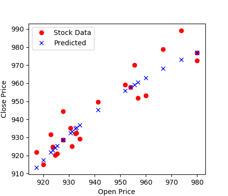
Once the data is imported, it can be analyzed with many different tools such as machine learning algorithms. Below is an example of using the data for analysis of correlation between open and close price of Google publicly traded shares.

Once the data is imported, it can be analyzed with many different tools such as machine learning algorithms. Below is an example of using the data for analysis of correlation between open and close price of Google stock.

(:toggle hide online2 button show="Show Python Regression Analysis":) (:div id=online2:) (:source lang=python:) from gekko import GEKKO import numpy as np import matplotlib.pyplot as plt import pandas as pd

1. Google stock

url = 'https://apmonitor.com/che263/uploads/Main/goog.csv'

1. import data with pandas

data = pd.read_csv(url) print(data['Close'][0:5]) print('min: '+str(min(data['Close'][0:20]))) print('max: '+str(max(data['Close'][0:20])))

1. GEKKO model

m = GEKKO()

1. input data

x = m.Param(value=np.array(data['Open']))

1. parameters to optimize

a = m.FV() a.STATUS=1 b = m.FV() b.STATUS=1 c = m.FV() c.STATUS=1

1. variables

y = m.CV(value=np.array(data['Close'])) y.FSTATUS=1

1. regression equation

m.Equation(y==b*m.exp(a*x)+c)

1. regression mode

m.options.IMODE = 2

1. optimize

m.options.solver = 1 m.solve(disp=True)

1. print parameters

print('Optimized, a = ' + str(a.value[0])) print('Optimized, b = ' + str(b.value[0])) print('Optimized, c = ' + str(c.value[0]))

1. plot data

plt.figure() plt.plot(data['Open'],data['Close'],'ro',label='Stock Data') plt.plot(x.value,y.value,'bx',label='Predicted') plt.xlabel('Open Price') plt.ylabel('Close Price') plt.legend() plt.show() (:sourceend:) (:divend:)

data = pd.read_csv(url)

stock = 'GOOG' url = 'https://apmonitor.com/che263/uploads/Main/goog.csv'

1. url = 'https://chart.finance.yahoo.com/table.csv?s='+stock

print('min: '+str(min(data['Close'][0:20]))) print('max: '+str(max(data['Close'][0:20])))

plt.plot(data['Open'][0:20]) plt.plot(data['Close'][0:20])

<iframe width="560" height="315" src="https://www.youtube.com/embed/pQv6zMlYJ0A" frameborder="0" allowfullscreen></iframe>

A common task for scientists and engineers is to analyze data from an external source that may be in a text or comma separated value (CSV) format. By importing the data into Python, data analysis such as statistics, trending, or calculations can be made to synthesize the information into relevant and actionable information. Tutorials below demonstrate how to import data (including online data), perform a basic analysis, trend the results, and export the results to another text file. Two examples are provided with Numpy and Pandas. Script files of the Python source code with sample data are below.

(:toggle hide online button show="Show Python Source":) (:div id=online:)

(:html:) <iframe width="560" height="315" src="//www.youtube.com/embed/Tq6rCWPdXoQ" frameborder="0" allowfullscreen></iframe> (:htmlend:)

Import Data and Analyze with Pandas

Python Data Analysis Example Source Code (Pandas)

<iframe width="560" height="315" src="https://www.youtube.com/embed/FXhED53VZ50" frameborder="0" allowfullscreen></iframe>

(:toggle hide pandas button show="Show Python Source":) (:div id=pandas:)

(:divend:)

(:toggle hide numpy button show="Show Python (NumPy) Source":)

Python Data Analysis Example Source Code (Numpy)

(:toggle hide numpy button show="Show Solution":) (:div id=numpy:)

1. Numpy (data import, manipulation, export)

1. Matplotlib (create trends)

data_file = np.genfromtxt('data_file.txt', delimiter=',')

1. create time vector from imported data (starts from index 0)

time = data_file[:,0]

sensors = data_file[:,1:5]

1. stack time and avg as column vectors

my_data = np.vstack((time,sensors.T,avg))

1. transpose data

my_data = my_data.T

1. save text file with comma delimiter

np.savetxt('export_from_python.txt',my_data,delimiter=',')

plt.plot(time/60.0,sensors[:,1],'ro') plt.plot(time/60.0,avg,'b.')

plt.legend(['Sensor 2','Average Sensors 1-4']) plt.xlabel('Time (min)')

1. show the figure on the screen (pauses execution until closed)

(:divend:)

(:html:) <iframe width="560" height="315" src="//www.youtube.com/embed/Tq6rCWPdXoQ" frameborder="0" allowfullscreen></iframe> (:htmlend:)

Import Data and Analyze with Pandas

• Python Data Analysis Example Source Code (Pandas)

(:html:) <iframe width="560" height="315" src="https://www.youtube.com/embed/FXhED53VZ50" frameborder="0" allowfullscreen></iframe> (:htmlend:)

(:toggle hide pandas button show="Show Python (Pandas) Source":) (:div id=pandas:) (:source lang=python:)

1. import Numpy, Pandas, and Matplotlib

import numpy as np import pandas as pd import matplotlib.pyplot as plt

1. load the data file

data_file = pd.read_csv('data_with_headers.csv')

1. create time vector from imported data

time = data_file['time']

1. parse good sensor data from imported data

sensors = data_file.ix[:,'s1':'s4']

1. display the first 6 sensor rows

print(sensors[0:6])

1. adjust time to start at zero by subtracting the
2. first element in the time vector (index = 0)

time = time - time[0]

1. calculate the average of the sensor readings

avg = np.mean(sensors,1) # over the 2nd dimension

1. export data

my_data = [time, sensors, avg] result = pd.concat(my_data,axis=1)

result.to_csv('result.csv')

1. result.to_excel('result.xlsx')

result.to_html('result.htm') result.to_clipboard()

1. generate a figure

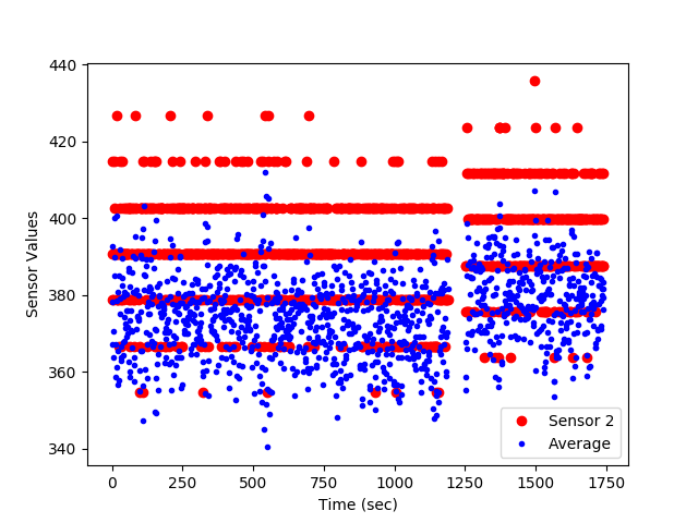
plt.figure(1) plt.plot(time,sensors['s1'],'r-') plt.plot(time,avg,'b.')

1. add text labels to the plot

plt.legend(['Sensor 2','Average']) plt.xlabel('Time (sec)') plt.ylabel('Sensor Values')

1. save the figure as a PNG file

plt.savefig('my_Python_plot.png')

1. show the figure on the screen

plt.show() (:sourceend:) (:divend:)

Import Online Data and Analyze

(:html:) <iframe width="560" height="315" src="https://www.youtube.com/embed/KzOEmMiPSjg" frameborder="0" allowfullscreen></iframe> (:htmlend:)

Below is an example of pulling data from an Internet source, such as financial information about a stock. The example shows how to request, parse, and display the financial data.

plt.show() (:sourceend:)

Import Data from an Internet Source

(:source lang=python:) import pandas as pd from matplotlib.finance import * import matplotlib.pyplot as plt try:

    import wget

except:

    # install wget if needed
    import pip
    pip.main(['install','wget'])
    import wget

1. stock ticker symbol

stock = 'GOOGL' url = 'https://chart.finance.yahoo.com/table.csv?s='+stock filename = wget.download(url)

1. rename file

from shutil import move move(filename,stock.lower()+'.csv')

1. import data with pandas

data = pd.read_csv(stock+'.csv') print(data['Close'][0:5]) print('min: '+str(min(data['Close'][0:30]))) print('max: '+str(max(data['Close'][0:30])))

1. plot data with pyplot

plt.figure() plt.plot(data['Open'][0:30]) plt.plot(data['Close'][0:30]) plt.xlabel('days ago') plt.ylabel('price')

(:source lang=python:)

1. import Numpy, Pandas, and Matplotlib

import numpy as np import pandas as pd import matplotlib.pyplot as plt

1. load the data file

data_file = pd.read_csv('data_with_headers.csv')

1. create time vector from imported data

time = data_file['time']

1. parse good sensor data from imported data

sensors = data_file.ix[:,'s1':'s4']

1. display the first 6 sensor rows

print(sensors[0:6])

1. adjust time to start at zero by subtracting the
2. first element in the time vector (index = 0)

time = time - time[0]

1. calculate the average of the sensor readings

avg = np.mean(sensors,1) # over the 2nd dimension

1. export data

my_data = [time, sensors, avg] result = pd.concat(my_data,axis=1)

result.to_csv('result.csv')

1. result.to_excel('result.xlsx')

result.to_html('result.htm') result.to_clipboard()

1. generate a figure

plt.figure(1) plt.plot(time,sensors['s1'],'r-') plt.plot(time,avg,'b.')

1. add text labels to the plot

plt.legend(['Sensor 2','Average']) plt.xlabel('Time (sec)') plt.ylabel('Sensor Values')

1. save the figure as a PNG file

plt.savefig('my_Python_plot.png')

1. show the figure on the screen

plt.show() (:sourceend:)

 print(sensors[0:6])

<iframe width="560" height="315" src="//www.youtube.com/embed/Tq6rCWPdXoQ" frameborder="0" allowfullscreen></iframe>

<iframe width="560" height="315" src="https://www.youtube.com/embed/FXhED53VZ50" frameborder="0" allowfullscreen></iframe>

<iframe width="560" height="315" src="https://www.youtube.com/embed/FXhED53VZ50" frameborder="0" allowfullscreen></iframe>

A common task for scientists and engineers is to analyze data from an external source that may be in a text or comma separated value (CSV) format. By importing the data into Python, data analysis such as statistics, trending, or calculations can be made to synthesize the information into relevant and actionable information. This tutorial demonstrates how to import data, perform a basic analysis, trend the results, and export the results to another text file. Two examples are provided with Numpy and Pandas. Script files of the Python source code with sample data are below.

• Python Data Analysis Example Source Code (Numpy)

• Python Data Analysis Example Source Code (Pandas)

Import Data and Analyze with Numpy

Import Data and Analyze with Pandas

• Python Data Analysis Example Source Code

(:html:) <iframe width="560" height="315" src="//www.youtube.com/embed/Tq6rCWPdXoQ" frameborder="0" allowfullscreen></iframe> (:htmlend:)

Source Code

 # import Numpy, Pandas, and Matplotlib
 import numpy as np
 import pandas as pd
 import matplotlib.pyplot as plt

 # load the data file
 data_file = pd.read_csv('data_with_headers.csv')

 # create time vector from imported data
 time = data_file['time']
 # parse good sensor data from imported data
 sensors = data_file.ix[:,'s1':'s4']

 # display the first 6 sensor rows
 print sensors[0:6]

 # adjust time to start at zero by subtracting the
 #  first element in the time vector (index = 0)
 time = time - time[0]

 # calculate the average of the sensor readings
 avg = np.mean(sensors,1) # over the 2nd dimension

 # export data
 my_data = [time, sensors, avg]
 result = pd.concat(my_data,axis=1)

 result.to_csv('result.csv')
 #result.to_excel('result.xlsx')
 result.to_html('result.htm')
 result.to_clipboard()

 # generate a figure
 plt.figure(1)
 plt.plot(time,sensors['s1'],'r-')
 plt.plot(time,avg,'b.')
 # add text labels to the plot
 plt.legend(['Sensor 2','Average'])
 plt.xlabel('Time (sec)')
 plt.ylabel('Sensor Values')
 # save the figure as a PNG file
 plt.savefig('my_Python_plot.png')
 # show the figure on the screen
 plt.show()

<iframe width="560" height="315" src="//www.youtube.com/embed/Tq6rCWPdXoQ" frameborder="0" allowfullscreen></iframe>

A common task for scientists and engineers is to analyze data from an external source that may be in a text or comma separated value (CSV) format. By importing the data into Python, data analysis such as statistics, trending, or calculations can be made to synthesize the information into relevant and actionable information. This tutorial demonstrates how to import data, perform a basic analysis, trend the results, and export the results to another text file. A script file of the Python source code with sample data is below.

• Python Data Analysis Example Source Code

This tutorial can also be completed with Excel and Matlab. Click on the appropriate link for additional information.

(:title Data Analysis with Python:) (:keywords big data, data analysis, Python, numpy, spreadsheet, nonlinear, optimization, engineering optimization, university course:) (:description Data Analysis with Python - Problem-Solving Techniques for Chemical Engineers at Brigham Young University:)

Python Data Analysis

(:html:) <iframe width="560" height="315" src="//www.youtube.com/embed/E56egH10RJA?list=PLLBUgWXdTBDi-E--rwBujaNkTejLNI6ap" frameborder="0" allowfullscreen></iframe> (:htmlend:)

(:html:)

 <div id="disqus_thread"></div>
    <script type="text/javascript">
        /* * * CONFIGURATION VARIABLES: EDIT BEFORE PASTING INTO YOUR WEBPAGE * * */
        var disqus_shortname = 'apmonitor'; // required: replace example with your forum shortname

        /* * * DON'T EDIT BELOW THIS LINE * * */
        (function() {
            var dsq = document.createElement('script'); dsq.type = 'text/javascript'; dsq.async = true;
            dsq.src = 'https://' + disqus_shortname + '.disqus.com/embed.js';
            (document.getElementsByTagName('head')[0] || document.getElementsByTagName('body')[0]).appendChild(dsq);
        })();
    </script>
    <noscript>Please enable JavaScript to view the <a href="https://disqus.com/?ref_noscript">comments powered by Disqus.</a></noscript>
    <a href="https://disqus.com" class="dsq-brlink">comments powered by <span class="logo-disqus">Disqus</span></a>

(:htmlend:)