Simulated annealing copies a phenomenon in nature--the annealing of solids--to optimize a complex system. Annealing refers to heating a solid and then cooling it slowly. Atoms then assume a nearly globally minimum energy state. In 1953 Metropolis created an algorithm to simulate the annealing process. The algorithm simulates a small random displacement of an atom that results in a change in energy. If the change in energy is negative, the energy state of the new configuration is lower and the new configuration is accepted. If the change in energy is positive, the new configuration has a higher energy state; however, it may still be accepted according to the Boltzmann probability factor:
$$P = \exp\left(\frac{-\Delta E}{k_b T}\right)$$
where kb is the Boltzmann constant and T is the current temperature. By examining this equation we should note two things: the probability is proportional to temperature--as the solid cools, the probability gets smaller; and inversely proportional to --as the change in energy is larger the probability of accepting the change gets smaller.
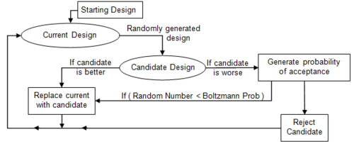
When applied to engineering design, an analogy is made between energy and the objective function. The design is started at a high “temperature”, where it has a high objective (we assume we are minimizing). Random perturbations are then made to the design. If the objective is lower, the new design is made the current design; if it is higher, it may still be accepted according the probability given by the Boltzmann factor. The Boltzmann probability is compared to a random number drawn from a uniform distribution between 0 and 1; if the random number is smaller than the Boltzmann probability, the configuration is accepted. This allows the algorithm to escape local minima.
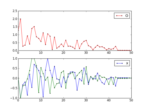
As the temperature is gradually lowered, the probability that a worse design is accepted becomes smaller. Typically at high temperatures the gross structure of the design emerges which is then refined at lower temperatures.
Although it can be used for continuous problems, simulated annealing is especially effective when applied to combinatorial or discrete problems. Although the algorithm is not guaranteed to find the best optimum, it will often find near optimum designs with many fewer design evaluations than other algorithms. (It can still be computationally expensive, however.) It is also an easy algorithm to implement.
Example Problem and Source Code
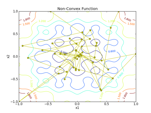
Find the minimum to the objective function
$$obj = 0.2 + x_1^2 + x_2^2 - 0.1 \, \cos \left( 6 \pi x_1 \right) - 0.1 \cos \left(6 \pi x_2\right)$$
by adjusting the values of `x_1` and `x_2`. You can download anneal.m and anneal.py files to retrieve example simulated annealing files in MATLAB and Python, respectively.
Download Simulated Annealing Example Files

# Import some other libraries that we'll need
# matplotlib and numpy packages must also be installed
import matplotlib
import numpy as np
import matplotlib.pyplot as plt
import random
import math
# define objective function
def f(x):
x1 = x[0]
x2 = x[1]
obj = 0.2 + x1**2 + x2**2 - 0.1*math.cos(6.0*3.1415*x1) - 0.1*math.cos(6.0*3.1415*x2)
return obj
# Start location
x_start = [0.8, -0.5]
# Design variables at mesh points
i1 = np.arange(-1.0, 1.0, 0.01)
i2 = np.arange(-1.0, 1.0, 0.01)
x1m, x2m = np.meshgrid(i1, i2)
fm = np.zeros(x1m.shape)
for i in range(x1m.shape[0]):
for j in range(x1m.shape[1]):
fm[i][j] = 0.2 + x1m[i][j]**2 + x2m[i][j]**2 \
- 0.1*math.cos(6.0*3.1415*x1m[i][j]) \
- 0.1*math.cos(6.0*3.1415*x2m[i][j])
# Create a contour plot
plt.figure()
# Specify contour lines
#lines = range(2,52,2)
# Plot contours
CS = plt.contour(x1m, x2m, fm)#,lines)
# Label contours
plt.clabel(CS, inline=1, fontsize=10)
# Add some text to the plot
plt.title('Non-Convex Function')
plt.xlabel('x1')
plt.ylabel('x2')
##################################################
# Simulated Annealing
##################################################
# Number of cycles
n = 50
# Number of trials per cycle
m = 50
# Number of accepted solutions
na = 0.0
# Probability of accepting worse solution at the start
p1 = 0.7
# Probability of accepting worse solution at the end
p50 = 0.001
# Initial temperature
t1 = -1.0/math.log(p1)
# Final temperature
t50 = -1.0/math.log(p50)
# Fractional reduction every cycle
frac = (t50/t1)**(1.0/(n-1.0))
# Initialize x
x = np.zeros((n+1,2))
x[0] = x_start
xi = np.zeros(2)
xi = x_start
na = na + 1.0
# Current best results so far
xc = np.zeros(2)
xc = x[0]
fc = f(xi)
fs = np.zeros(n+1)
fs[0] = fc
# Current temperature
t = t1
# DeltaE Average
DeltaE_avg = 0.0
for i in range(n):
print('Cycle: ' + str(i) + ' with Temperature: ' + str(t))
for j in range(m):
# Generate new trial points
xi[0] = xc[0] + random.random() - 0.5
xi[1] = xc[1] + random.random() - 0.5
# Clip to upper and lower bounds
xi[0] = max(min(xi[0],1.0),-1.0)
xi[1] = max(min(xi[1],1.0),-1.0)
DeltaE = abs(f(xi)-fc)
if (f(xi)>fc):
# Initialize DeltaE_avg if a worse solution was found
# on the first iteration
if (i==0 and j==0): DeltaE_avg = DeltaE
# objective function is worse
# generate probability of acceptance
p = math.exp(-DeltaE/(DeltaE_avg * t))
# determine whether to accept worse point
if (random.random()<p):
# accept the worse solution
accept = True
else:
# don't accept the worse solution
accept = False
else:
# objective function is lower, automatically accept
accept = True
if (accept==True):
# update currently accepted solution
xc[0] = xi[0]
xc[1] = xi[1]
fc = f(xc)
# increment number of accepted solutions
na = na + 1.0
# update DeltaE_avg
DeltaE_avg = (DeltaE_avg * (na-1.0) + DeltaE) / na
# Record the best x values at the end of every cycle
x[i+1][0] = xc[0]
x[i+1][1] = xc[1]
fs[i+1] = fc
# Lower the temperature for next cycle
t = frac * t
# print solution
print('Best solution: ' + str(xc))
print('Best objective: ' + str(fc))
plt.plot(x[:,0],x[:,1],'y-o')
plt.savefig('contour.png')
fig = plt.figure()
ax1 = fig.add_subplot(211)
ax1.plot(fs,'r.-')
ax1.legend(['Objective'])
ax2 = fig.add_subplot(212)
ax2.plot(x[:,0],'b.-')
ax2.plot(x[:,1],'g--')
ax2.legend(['x1','x2'])
# Save the figure as a PNG
plt.savefig('iterations.png')
plt.show()
clear;
close all;
%% Generate a contour plot
% Start location
x_start = [0.8, -0.5];
% Design variables at mesh points
i1 = -1.0:0.01:1.0;
i2 = -1.0:0.01:1.0;
[x1m, x2m] = meshgrid(i1, i2);
fm = 0.2 + x1m.^2 + x2m.^2 - 0.1*cos(6.0*pi*x1m) - 0.1*cos(6.0*pi*x2m);
% Contour Plot
fig = figure(1);
[C,h] = contour(x1m,x2m,fm);
clabel(C,h,'Labelspacing',250);
title('Simulated Annealing');
xlabel('x1');
ylabel('x2');
hold on;
%% Simulated Annealing
% Number of cycles
n = 50;
% Number of trials per cycle
m = 50;
% Number of accepted solutions
na = 0.0;
% Probability of accepting worse solution at the start
p1 = 0.7;
% Probability of accepting worse solution at the end
p50 = 0.001;
% Initial temperature
t1 = -1.0/log(p1);
% Final temperature
t50 = -1.0/log(p50);
% Fractional reduction every cycle
frac = (t50/t1)^(1.0/(n-1.0));
% Initialize x
x = zeros(n+1,2);
x(1,:) = x_start;
xi = x_start;
na = na + 1.0;
% Current best results so far
% xc = x(1,:);
fc = f(xi);
fs = zeros(n+1,1);
fs(1,:) = fc;
% Current temperature
t = t1;
% DeltaE Average
DeltaE_avg = 0.0;
for i=1:n
disp(['Cycle: ',num2str(i),' with Temperature: ',num2str(t)])
xc(1) = x(i,1);
xc(2) = x(i,2);
for j=1:m
% Generate new trial points
xi(1) = xc(1) + rand() - 0.5;
xi(2) = xc(2) + rand() - 0.5;
% Clip to upper and lower bounds
xi(1) = max(min(xi(1),1.0),-1.0);
xi(2) = max(min(xi(2),1.0),-1.0);
DeltaE = abs(f(xi)-fc);
if (f(xi)>fc)
% Initialize DeltaE_avg if a worse solution was found
% on the first iteration
if (i==1 && j==1)
DeltaE_avg = DeltaE;
end
% objective function is worse
% generate probability of acceptance
p = exp(-DeltaE/(DeltaE_avg * t));
% % determine whether to accept worse point
if (rand()<p)
% accept the worse solution
accept = true;
else
% don't accept the worse solution
accept = false;
end
else
% objective function is lower, automatically accept
accept = true;
end
% accept
if (accept==true)
% update currently accepted solution
xc(1) = xi(1);
xc(2) = xi(2);
fc = f(xc);
xa(j,1) = xc(1);
xa(j,2) = xc(2);
fa(j) = f(xc);
% increment number of accepted solutions
na = na + 1.0;
% update DeltaE_avg
DeltaE_avg = (DeltaE_avg * (na-1.0) + DeltaE) / na;
else
fa(j) = 0.0;
end
end
% cycle)
fa_Min_Index = find(nonzeros(fa) == min(nonzeros(fa)));
if isempty(fa_Min_Index) == 0
x(i+1,1) = xa(fa_Min_Index,1);
x(i+1,2) = xa(fa_Min_Index,2);
fs(i+1) = fa(fa_Min_Index);
else
x(i+1,1) = x(i,1);
x(i+1,2) = x(i,2);
fs(i+1) = fs(i);
end
% Lower the temperature for next cycle
t = frac * t;
fa = 0.0;
end
% print solution
disp(['Best candidate: ',num2str(xc)])
disp(['Best solution: ',num2str(fc)])
plot(x(:,1),x(:,2),'r-o')
saveas(fig,'contour','png')
fig = figure(2);
subplot(2,1,1)
plot(fs,'r.-')
legend('Objective')
subplot(2,1,2)
hold on
plot(x(:,1),'b.-')
plot(x(:,2),'g.-')
legend('x_1','x_2')
% Save the figure as a PNG
saveas(fig,'iterations','png')
Save as f.m
x1 = x(1);
x2 = x(2);
obj = 0.2 + x1^2 + x2^2 - 0.1*cos(6.0*pi*x1) - 0.1*cos(6.0*pi*x2);
end