Transformers have revolutionized the field of Natural Language Processing (NLP) and are increasingly being used in time-series forecasting. Originally introduced in the paper Attention Is All You Need, transformers have become the backbone of many state-of-the-art language models like BERT, GPT, and others. This page uses Keras / TensorFlow and code is also available with the PyTorch package.
Transformers in Large Language Models (LLM)
Transformers in LLMs like GPT and BERT use self-attention mechanisms to process text. They are capable of capturing contextual information from the entire text input, making them effective for a variety of NLP tasks.
Basic Usage Example with the transformers package
# Using a pre-trained model
generator = pipeline('text-generation', model='gpt2')
generated_text = generator("Today is a beautiful day and", max_length=30)
print(generated_text)
Transformers in Time-Series Forecasting
In time-series forecasting, transformers are used to analyze sequential data, capturing temporal dependencies. They are particularly effective in scenarios where long-range dependencies are important.
Data Generation: This section of the script is responsible for creating synthetic time-series data. It uses a sine function to generate a sequence of data points, mimicking a real-world time-series dataset. The data is split into sequences of a specified length, with each sequence used to predict the next point in the series. This mimics a common scenario in time-series analysis where past data is used to predict future values.
# Generating synthetic time-series data
def generate_data(size=1000, sequence_length=10):
data = np.sin(np.linspace(0, 10 * np.pi, size)) # Sine wave data
sequences = [data[i:i+sequence_length] for i in range(size-sequence_length)]
next_points = data[sequence_length:]
return np.array(sequences), next_points
Custom Dataset Class: This part defines a custom Dataset class for handling the time-series data using Keras utilities. The class, TimeSeriesDataset, uses tf.keras.utils.Sequence to efficiently handle batching and shuffling of the data for training.
import tensorflow as tf
from tensorflow.keras.utils import Sequence
class TimeSeriesDataset(Sequence):
def __init__(self, sequences, next_points, batch_size=32, shuffle=True):
self.sequences = sequences
self.next_points = next_points
self.batch_size = batch_size
self.shuffle = shuffle
self.indices = np.arange(len(self.sequences))
self.on_epoch_end()
def __len__(self):
return int(np.ceil(len(self.sequences) / self.batch_size))
def __getitem__(self, index):
batch_indices = self.indices[index*self.batch_size:(index+1)*self.batch_size]
X = self.sequences[batch_indices]
y = self.next_points[batch_indices]
return X, y
def on_epoch_end(self):
if self.shuffle:
np.random.shuffle(self.indices)
Transformer Model Definition: In this section, a transformer model specifically tailored for numerical time-series data is defined using Keras and TensorFlow. The model projects each time-step into a higher dimensional space, applies transformer encoder blocks to capture temporal dependencies, and then flattens the output for the final prediction.
from tensorflow.keras.layers import Dense, LayerNormalization, Dropout, MultiHeadAttention, Flatten, Input, Lambda
from tensorflow.keras.models import Model
# Transformer model definition using Keras
def create_transformer_model(sequence_length, d_model=32, num_heads=2, ff_dim=64, num_layers=1, dropout=0.1):
inputs = Input(shape=(sequence_length,))
# Wrap tf.expand_dims in a Lambda layer to work with Keras tensors
x = Lambda(lambda x: tf.expand_dims(x, axis=-1))(inputs) # Shape: (batch, sequence_length, 1)
x = Dense(d_model)(x)
for _ in range(num_layers):
attn_output = MultiHeadAttention(num_heads=num_heads, key_dim=d_model, dropout=dropout)(x, x)
attn_output = Dropout(dropout)(attn_output)
x = LayerNormalization(epsilon=1e-6)(x + attn_output)
ff = Dense(ff_dim, activation="relu")(x)
ff = Dense(d_model)(ff)
ff = Dropout(dropout)(ff)
x = LayerNormalization(epsilon=1e-6)(x + ff)
x = Flatten()(x)
outputs = Dense(1)(x)
model = Model(inputs=inputs, outputs=outputs)
return model
Data Preparation for Training: This part of the script involves instantiating the dataset using the custom TimeSeriesDataset class. The dataset is then ready to be fed into the training process.
sequences, next_points = generate_data()
dataset = TimeSeriesDataset(sequences, next_points, batch_size=32)
Model Training: Here, the model is compiled and trained using the time-series data. The model uses Mean Squared Error (MSE) as the loss function and the Adam optimizer for training. Training is handled via Keras's high-level API.
from tensorflow.keras.optimizers import Adam
# Create and compile the model
model = create_transformer_model(sequence_length=10, d_model=32, num_heads=2, ff_dim=64, num_layers=1)
model.compile(optimizer=Adam(learning_rate=0.001), loss='mse')
# Train the model
model.fit(dataset, epochs=9)
  Epoch 1/9
  ...
  Epoch 9/9
Prediction: In the final part of the script, the trained model is used to make a prediction. It takes a sequence from the dataset and predicts the next data point, demonstrating the model's ability to perform time-series forecasting.
# Predict the next point after a sequence
test_seq = np.array(sequences[0])
predicted_point = model.predict(np.expand_dims(test_seq, axis=0))
print("Predicted next point:", predicted_point[0, 0])
Predicted next point: 0.3071648
The complete code is given below on generating synthetic data, training the transformer, and predicting the next point as a time-series forecast.
import tensorflow as tf
from tensorflow.keras.layers import Dense, LayerNormalization, Dropout, MultiHeadAttention, Flatten, Input, Lambda
from tensorflow.keras.models import Model
from tensorflow.keras.optimizers import Adam
from tensorflow.keras.utils import Sequence
# Generating synthetic time-series data
def generate_data(size=1000, sequence_length=10):
data = np.sin(np.linspace(0, 10 * np.pi, size)) # Sine wave data
sequences = np.array([data[i:i+sequence_length] for i in range(size - sequence_length)])
next_points = data[sequence_length:]
return sequences, next_points
# Custom dataset class using Keras Sequence
class TimeSeriesDataset(Sequence):
def __init__(self, sequences, next_points, batch_size=32, shuffle=True):
self.sequences = sequences
self.next_points = next_points
self.batch_size = batch_size
self.shuffle = shuffle
self.indices = np.arange(len(self.sequences))
self.on_epoch_end()
def __len__(self):
return int(np.ceil(len(self.sequences) / self.batch_size))
def __getitem__(self, index):
batch_indices = self.indices[index * self.batch_size:(index + 1) * self.batch_size]
X = self.sequences[batch_indices]
y = self.next_points[batch_indices]
return X, y
def on_epoch_end(self):
if self.shuffle:
np.random.shuffle(self.indices)
# Transformer model definition using Keras
def create_transformer_model(sequence_length, d_model=32, num_heads=2, ff_dim=64, num_layers=1, dropout=0.1):
inputs = Input(shape=(sequence_length,))
# Wrap tf.expand_dims in a Lambda layer to work with Keras tensors
x = Lambda(lambda x: tf.expand_dims(x, axis=-1))(inputs) # Shape: (batch, sequence_length, 1)
x = Dense(d_model)(x)
for _ in range(num_layers):
attn_output = MultiHeadAttention(num_heads=num_heads, key_dim=d_model, dropout=dropout)(x, x)
attn_output = Dropout(dropout)(attn_output)
x = LayerNormalization(epsilon=1e-6)(x + attn_output)
ff = Dense(ff_dim, activation="relu")(x)
ff = Dense(d_model)(ff)
ff = Dropout(dropout)(ff)
x = LayerNormalization(epsilon=1e-6)(x + ff)
x = Flatten()(x)
outputs = Dense(1)(x)
model = Model(inputs=inputs, outputs=outputs)
return model
# Prepare data
sequences, next_points = generate_data()
dataset = TimeSeriesDataset(sequences, next_points, batch_size=32)
# Create and compile the model
model = create_transformer_model(sequence_length=10, d_model=32, num_heads=2, ff_dim=64, num_layers=1)
model.compile(optimizer=Adam(learning_rate=0.001), loss='mse')
# Train the model
model.fit(dataset, epochs=9)
# Predict the next point after a sequence
test_seq = np.array(sequences[0])
predicted_point = model.predict(np.expand_dims(test_seq, axis=0))
print("Predicted next point:", predicted_point[0, 0])
Exercise: Transformer Forecast with TCLab
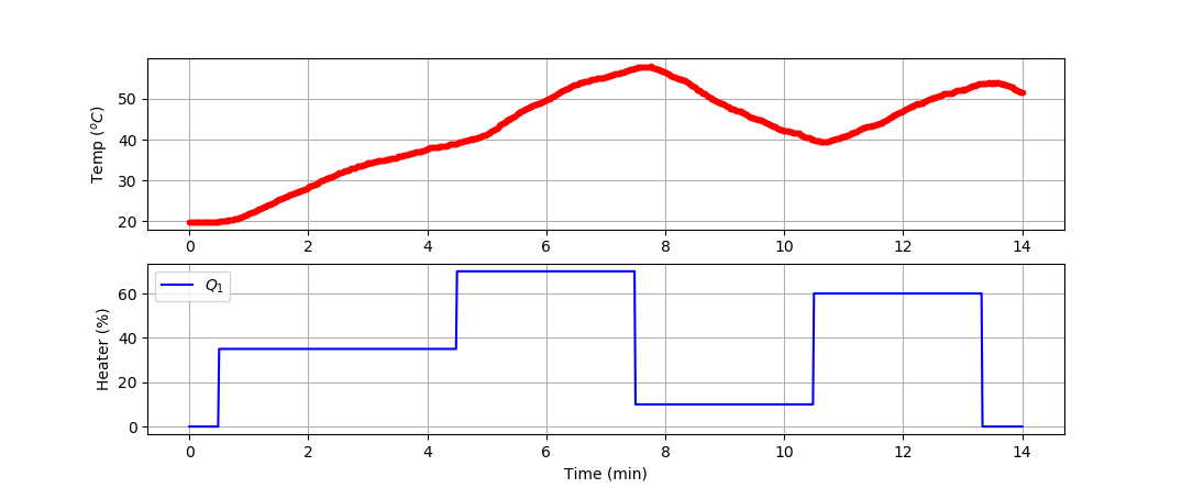
Develop a model of the dynamic temperature response of the TCLab and compare the Transformer model prediction to measurements. Use the 4 hours of dynamic data from a TCLab (14400 data points = 1 second sample rate for 4 hours) for training and generate new data (840 data points = 1 second sample rate for 14 min) for validation (see sample validation data).
import numpy as np
import matplotlib.pyplot as plt
import pandas as pd
import tclab
import time
n = 840 # Number of second time points (14 min)
tm = np.linspace(0,n,n+1) # Time values
lab = tclab.TCLab()
T1 = [lab.T1]
T2 = [lab.T2]
Q1 = np.zeros(n+1)
Q2 = np.zeros(n+1)
Q1[30:] = 35.0
Q1[270:] = 70.0
Q1[450:] = 10.0
Q1[630:] = 60.0
Q1[800:] = 0.0
for i in range(n):
lab.Q1(Q1[i])
lab.Q2(Q2[i])
time.sleep(1)
print(Q1[i],lab.T1)
T1.append(lab.T1)
T2.append(lab.T2)
lab.close()
# Save data file
data = np.vstack((tm,Q1,Q2,T1,T2)).T
np.savetxt('tclab_data.csv',data,delimiter=',',\
header='Time,Q1,Q2,T1,T2',comments='')
# Create Figure
plt.figure(figsize=(10,7))
ax = plt.subplot(2,1,1)
ax.grid()
plt.plot(tm/60.0,T1,'r.',label=r'$T_1$')
plt.ylabel(r'Temp ($^oC$)')
ax = plt.subplot(2,1,2)
ax.grid()
plt.plot(tm/60.0,Q1,'b-',label=r'$Q_1$')
plt.ylabel(r'Heater (%)')
plt.xlabel('Time (min)')
plt.legend()
plt.savefig('tclab_data.png')
plt.show()
Use the measured temperature and heater values to predict the next temperature value with a Transformer model. Validate the model with a new data set in a predictive and forecast mode. The predictive mode predicts one step ahead while the forecast does not use temperature measurements to generate the predictions.
Solution with Transformer Model with TCLab Data


Further Reading
- Attention Is All You Need - Seminal paper introducing transformers.
- BERT: Pre-training of Deep Bidirectional Transformers for Language Understanding - Paper introducing BERT.
- Language Models are Few-Shot Learners - Paper on the GPT-3 model.
- Transformers in Time-Series: A Survey
- How to Apply Transformers to Time Series Models - Medium Article by Intel Tech.
- Time Series Transformer - Documentation on HuggingFace.
✅ Knowledge Check
1. What is the primary mechanism that transformers use to process text in language models?
- Incorrect. Transformers use self-attention mechanisms to process text.
- Correct. Transformers use self-attention mechanisms to process text.
- Incorrect. Transformers use self-attention mechanisms to process text.
2. Why are transformers effective in time-series forecasting?
- Correct. Transformers are effective because they can capture long-range dependencies in sequential data.
- Incorrect. The effectiveness of transformers is not primarily due to reduced data requirements.
- Incorrect. This is a disadvantage of LSTM models that do not capture long-range dependencies because of vanishing gradients.