Dynamic Optimization

         lw=3,label=r'$T_1$ sensor')

         lw=3,label=r'$T_2$ sensor')

         lw=3,label=r'$Q_1$')

         lw=3,label=r'$Q_2$')

Virtual TCLab on Google Colab

Note: Switch to make_mp4 = True to make an MP4 movie animation. This requires imageio and ffmpeg (install available through Python). It creates a folder named figures in your run directory. You can delete this folder after the run is complete.

1. Make an MP4 animation?

make_mp4 = False if make_mp4:

    import imageio  # required to make animation
    import os
    try:
        os.mkdir('./figures')
    except:
        pass

1. change to remote=True for MacOS

tau = m.FV(value=5,name='tau')

tau.LOWER = 4 tau.UPPER = 8

        m.solve(disp=True) 

        if make_mp4:
            filename='./figures/plot_str(i+10000).png'
            plt.savefig(filename)

    # generate mp4 from png figures in batches of 350
    if make_mp4:
        images = []
        iset = 0
        for i in range(1,n):
            filename='./figures/plot_str(i+10000).png'
            images.append(imageio.imread(filename))
            if ((i+1)%350)==0:
                imageio.mimsave('results_str(iset).mp4', images)
                iset += 1
                images = []
        if images!=[]:
            imageio.mimsave('results_str(iset).mp4', images)

(:toggle hide gekko_labEm button show="Lab E: Python GEKKO Moving Horizon Estimation":) (:div id=gekko_labEm:)

import numpy as np import time import matplotlib.pyplot as plt import random

1. get gekko package with:
2. pip install gekko

from gekko import GEKKO

1. get tclab package with:
2. pip install tclab

from tclab import TCLab

1. Connect to Arduino

a = TCLab()

1. Final time

tf = 10 # min

1. number of data points (1 pt every 3 seconds)

n = tf * 20 + 1

1. Configure heater levels
2. Percent Heater (0-100%)

Q1s = np.zeros(n) Q2s = np.zeros(n)

1. Heater random steps every 50 sec
2. Alternate steps by Q1 and Q2

Q1s[3:] = 100.0 Q1s[50:] = 0.0 Q1s[100:] = 80.0

Q2s[25:] = 60.0 Q2s[75:] = 100.0 Q2s[125:] = 25.0

1. rapid, random changes every 5 cycles between 50 and 100

for i in range(130,180):

    if i%10==0:
        Q1s[i:i+10] = random.random() * 100.0
    if (i+5)%10==0:
        Q2s[i:i+10] = random.random() * 100.0

1. Record initial temperatures (degC)

T1m = a.T1 * np.ones(n) T2m = a.T2 * np.ones(n)

1. Store MHE values for plots

Tmhe1 = T1m[0] * np.ones(n) Tmhe2 = T2m[0] * np.ones(n) Umhe = 10.0 * np.ones(n) taumhe = 5.0 * np.ones(n) amhe1 = 0.01 * np.ones(n) amhe2 = 0.0075 * np.ones(n)

1. Initialize Model as Estimator

2. Use remote=False for local solve (Windows, Linux, ARM)
3. remote=True for remote solve (All platforms)

m = GEKKO(name='tclab-mhe',remote=False)

1. 60 second time horizon, 20 steps

m.time = np.linspace(0,60,21)

1. Parameters to Estimate

U = m.FV(value=10,name='u') U.STATUS = 0 # don't estimate initially U.FSTATUS = 0 # no measurements U.DMAX = 1 U.LOWER = 5 U.UPPER = 15

tau = m.FV(value=20,name='tau') tau.STATUS = 0 # don't estimate initially tau.FSTATUS = 0 # no measurements tau.DMAX = 1 tau.LOWER = 15 tau.UPPER = 25

alpha1 = m.FV(value=0.01,name='a1') # W / % heater alpha1.STATUS = 0 # don't estimate initially alpha1.FSTATUS = 0 # no measurements alpha1.DMAX = 0.001 alpha1.LOWER = 0.003 alpha1.UPPER = 0.03

alpha2 = m.FV(value=0.0075,name='a2') # W / % heater alpha2.STATUS = 0 # don't estimate initially alpha2.FSTATUS = 0 # no measurements alpha2.DMAX = 0.001 alpha2.LOWER = 0.002 alpha2.UPPER = 0.02

1. Measured inputs

Q1 = m.MV(value=0,name='q1') Q1.STATUS = 0 # don't estimate Q1.FSTATUS = 1 # receive measurement

Q2 = m.MV(value=0,name='q2') Q2.STATUS = 0 # don't estimate Q2.FSTATUS = 1 # receive measurement

1. State variables

TH1 = m.SV(value=T1m[0],name='th1') TH2 = m.SV(value=T2m[0],name='th2')

1. Measurements for model alignment

TC1 = m.CV(value=T1m[0],name='tc1') TC1.STATUS = 1 # minimize error between simulation and measurement TC1.FSTATUS = 1 # receive measurement TC1.MEAS_GAP = 0.1 # measurement deadband gap TC1.LOWER = 0 TC1.UPPER = 200

TC2 = m.CV(value=T2m[0],name='tc2') TC2.STATUS = 1 # minimize error between simulation and measurement TC2.FSTATUS = 1 # receive measurement TC2.MEAS_GAP = 0.1 # measurement deadband gap TC2.LOWER = 0 TC2.UPPER = 200

Ta = m.Param(value=23.0+273.15) # K mass = m.Param(value=4.0/1000.0) # kg Cp = m.Param(value=0.5*1000.0) # J/kg-K A = m.Param(value=10.0/100.0**2) # Area not between heaters in m^2 As = m.Param(value=2.0/100.0**2) # Area between heaters in m^2 eps = m.Param(value=0.9) # Emissivity sigma = m.Const(5.67e-8) # Stefan-Boltzmann

1. Heater temperatures

T1 = m.Intermediate(TH1+273.15) T2 = m.Intermediate(TH2+273.15)

1. Heat transfer between two heaters

Q_C12 = m.Intermediate(U*As*(T2-T1)) # Convective Q_R12 = m.Intermediate(eps*sigma*As*(T2**4-T1**4)) # Radiative

1. Semi-fundamental correlations (energy balances)

m.Equation(TH1.dt() == (1.0/(mass*Cp))*(U*A*(Ta-T1) + eps * sigma * A * (Ta**4 - T1**4) + Q_C12 + Q_R12 + alpha1*Q1))

m.Equation(TH2.dt() == (1.0/(mass*Cp))*(U*A*(Ta-T2) + eps * sigma * A * (Ta**4 - T2**4) - Q_C12 - Q_R12 + alpha2*Q2))

1. Empirical correlations (lag equations to emulate conduction)

m.Equation(tau * TC1.dt() == -TC1 + TH1) m.Equation(tau * TC2.dt() == -TC2 + TH2)

1. Global Options

m.options.IMODE = 5 # MHE m.options.EV_TYPE = 2 # Objective type m.options.NODES = 3 # Collocation nodes m.options.SOLVER = 3 # IPOPT m.options.COLDSTART = 1 # COLDSTART on first cycle

1. Create plot

plt.figure(figsize=(10,7)) plt.ion() plt.show()

1. Main Loop

start_time = time.time() prev_time = start_time tm = np.zeros(n)

try:

    for i in range(1,n):
        # Sleep time
        sleep_max = 3.0
        sleep = sleep_max - (time.time() - prev_time)
        if sleep>=0.01:
            time.sleep(sleep-0.01)
        else:
            time.sleep(0.01)

        # Record time and change in time
        t = time.time()
        dt = t - prev_time
        prev_time = t
        tm[i] = t - start_time

        # Read temperatures in Celsius 
        T1m[i] = a.T1
        T2m[i] = a.T2

        # Insert measurements
        TC1.MEAS = T1m[i]
        TC2.MEAS = T2m[i]
        Q1.MEAS = Q1s[i-1]
        Q2.MEAS = Q2s[i-1]

        # Start estimating U after 10 cycles (20 sec)
        if i==10:
            U.STATUS = 1
            tau.STATUS = 1
            alpha1.STATUS = 1
            alpha2.STATUS = 1

        # Predict Parameters and Temperatures with MHE
        m.solve() 

        if m.options.APPSTATUS == 1:
            # Retrieve new values
            Tmhe1[i] = TC1.MODEL
            Tmhe2[i] = TC2.MODEL
            Umhe[i]  = U.NEWVAL
            taumhe[i] = tau.NEWVAL
            amhe1[i] = alpha1.NEWVAL
            amhe2[i] = alpha2.NEWVAL
        else:
            # Solution failed, copy prior solution
            Tmhe1[i] = Tmhe1[i-1]
            Tmhe2[i] = Tmhe1[i-1]
            Umhe[i]  = Umhe[i-1]
            taumhe[i] = taumhe[i-1]
            amhe1[i] = amhe1[i-1]
            amhe2[i] = amhe2[i-1]

        # Write new heater values (0-100)
        a.Q1(Q1s[i])
        a.Q2(Q2s[i])

        # Plot
        plt.clf()
        ax=plt.subplot(3,1,1)
        ax.grid()
        plt.plot(tm[0:i],T1m[0:i],'ro',label=r'$T_1$ measured')
        plt.plot(tm[0:i],Tmhe1[0:i],'k-',label=r'$T_1$ MHE')
        plt.plot(tm[0:i],T2m[0:i],'bx',label=r'$T_2$ measured')
        plt.plot(tm[0:i],Tmhe2[0:i],'k--',label=r'$T_2$ MHE')
        plt.ylabel('Temperature (degC)')
        plt.legend(loc=2)
        ax=plt.subplot(3,1,2)
        ax.grid()
        plt.plot(tm[0:i],Umhe[0:i],'k-',label='Heat Transfer Coeff')
        plt.plot(tm[0:i],taumhe[0:i],'g:',label='Time Constant')        
        plt.plot(tm[0:i],amhe1[0:i]*1000,'r--',label=r'$\alpha_1$x1000')
        plt.plot(tm[0:i],amhe2[0:i]*1000,'b--',label=r'$\alpha_2$x1000')
        plt.ylabel('Parameters')
        plt.legend(loc='best')
        ax=plt.subplot(3,1,3)
        ax.grid()
        plt.plot(tm[0:i],Q1s[0:i],'r-',label=r'$Q_1$')
        plt.plot(tm[0:i],Q2s[0:i],'b:',label=r'$Q_2$')
        plt.ylabel('Heaters')
        plt.xlabel('Time (sec)')
        plt.legend(loc='best')
        plt.draw()
        plt.pause(0.05)

    # Turn off heaters
    a.Q1(0)
    a.Q2(0)
    # Save figure
    plt.savefig('tclab_mhe.png')

1. Allow user to end loop with Ctrl-C

except KeyboardInterrupt:

    # Disconnect from Arduino
    a.Q1(0)
    a.Q2(0)
    print('Shutting down')
    a.close()
    plt.savefig('tclab_mhe.png')

1. Make sure serial connection still closes when there's an error

except:

    # Disconnect from Arduino
    a.Q1(0)
    a.Q2(0)
    print('Error: Shutting down')
    a.close()
    plt.savefig('tclab_mhe.png')
    raise

import numpy as np import matplotlib.pyplot as plt import pandas as pd from gekko import GEKKO

1. Import or generate data

filename = 'tclab_dyn_data2.csv' try:

    data = pd.read_csv(filename)

except:

    url = 'https://apmonitor.com/do/uploads/Main/tclab_dyn_data2.txt'
    data = pd.read_csv(url)

1. Create GEKKO Model

m = GEKKO() m.time = data['Time'].values

1. Parameters to Estimate

U = m.FV(value=10,lb=1,ub=20) tau = m.FV(value=20,lb=15,ub=25) alpha1 = m.FV(value=0.01,lb=0.003,ub=0.03) # W / % heater alpha2 = m.FV(value=0.005,lb=0.002,ub=0.02) # W / % heater

1. STATUS=1 allows solver to adjust parameter

U.STATUS = 1 tau.STATUS = 1 alpha1.STATUS = 1 alpha2.STATUS = 1

1. Measured inputs

Q1 = m.MV(value=data['H1'].values) Q2 = m.MV(value=data['H2'].values)

1. State variables

TH1 = m.SV(value=data['T1'].values) TH2 = m.SV(value=data['T2'].values)

1. Measurements for model alignment

TC1 = m.CV(value=data['T1'].values,lb=0,ub=200) TC1.FSTATUS = 1 # minimize fstatus * (meas-pred)^2

TC2 = m.CV(value=data['T2'].values,lb=0,ub=200) TC2.FSTATUS = 1 # minimize fstatus * (meas-pred)^2

Ta = m.Param(value=19.0+273.15) # K mass = m.Param(value=4.0/1000.0) # kg Cp = m.Param(value=0.5*1000.0) # J/kg-K A = m.Param(value=10.0/100.0**2) # Area not between heaters in m^2 As = m.Param(value=2.0/100.0**2) # Area between heaters in m^2 eps = m.Param(value=0.9) # Emissivity sigma = m.Const(5.67e-8) # Stefan-Boltzmann

1. Heater temperatures in Kelvin

T1 = m.Intermediate(TH1+273.15) T2 = m.Intermediate(TH2+273.15)

1. Heat transfer between two heaters

Q_C12 = m.Intermediate(U*As*(T2-T1)) # Convective Q_R12 = m.Intermediate(eps*sigma*As*(T2**4-T1**4)) # Radiative

1. Semi-fundamental correlations (energy balances)

m.Equation(TH1.dt() == (1.0/(mass*Cp))*(U*A*(Ta-T1) + eps * sigma * A * (Ta**4 - T1**4) + Q_C12 + Q_R12 + alpha1*Q1))

m.Equation(TH2.dt() == (1.0/(mass*Cp))*(U*A*(Ta-T2) + eps * sigma * A * (Ta**4 - T2**4) - Q_C12 - Q_R12 + alpha2*Q2))

1. Empirical correlations (lag equations to emulate conduction)

m.Equation(tau * TC1.dt() == -TC1 + TH1) m.Equation(tau * TC2.dt() == -TC2 + TH2)

1. Options

m.options.IMODE = 5 # MHE m.options.EV_TYPE = 2 # Objective type m.options.NODES = 2 # Collocation nodes m.options.SOLVER = 3 # IPOPT

1. Solve

m.solve(disp=True)

1. Parameter values

print('U : ' + str(U.value[0])) print('tau : ' + str(tau.value[0])) print('alpha1: ' + str(alpha1.value[0])) print('alpha2: ' + str(alpha2.value[0]))

1. Create plot

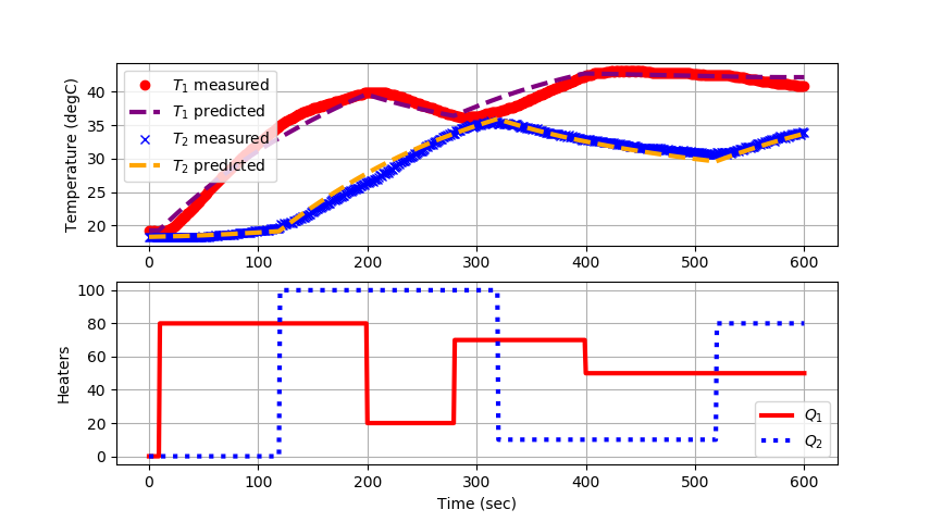
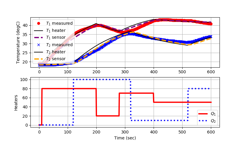
plt.figure() ax=plt.subplot(2,1,1) ax.grid() plt.plot(data['Time'],data['T1'],'ro',label=r'$T_1$ measured') plt.plot(m.time,TH1.value,'k-',label=r'$T_1$ heater') plt.plot(m.time,TC1.value,color='purple',linestyle=, linewidth=3,label=r'$T_1$ sensor') plt.plot(data['Time'],data['T2'],'bx',label=r'$T_2$ measured') plt.plot(m.time,TH2.value,'k-',label=r'$T_2$ heater') plt.plot(m.time,TC2.value,color='orange',linestyle=, linewidth=3,label=r'$T_2$ sensor') plt.ylabel('Temperature (degC)') plt.legend(loc=2) ax=plt.subplot(2,1,2) ax.grid() plt.plot(data['Time'],data['H1'],'r-', linewidth=3,label=r'$Q_1$') plt.plot(data['Time'],data['H2'],'b:', linewidth=3,label=r'$Q_2$') plt.ylabel('Heaters') plt.xlabel('Time (sec)') plt.legend(loc='best') plt.show()

The TCLab is a hands-on application of machine learning and advanced temperature control with two heaters and two temperature sensors. The labs reinforce principles of model development, estimation, and advanced control methods. This is the fifth exercise and it involves estimating parameters in a multi-variate energy balance model with added empirical elements. The predictions are aligned to the measured values through an optimizer that adjusts the parameters to minimize a sum of squared error or sum of absolute values objective. This lab builds upon the TCLab C by using the estimation of parameters in an energy balance but also adding additional equations that give a 2nd order response. The 2nd order response comes from splitting the finite element model of the heaters and temperature sensors. This creates a total of 4 differential equations with parameters that are adjusted to minimize the difference between the predicted and measured temperatures.

Attach:tclab_mhe_hybrid.mp4

  <source src="/do/uploads/Main/tclab_mhe_hybrid.mp4" type="video/mp4">

(:toggle hide gekko_labCm button show="Lab E: Python GEKKO Moving Horizon Estimation":)

(:title TCLab E - Hybrid Model Estimation:) (:keywords Arduino, Hybrid, Parameter, Regression, temperature, control, process control, course:) (:description Regression of Parameters in Multivariate (MIMO) Energy Balance with Empirical Elements using Arduino Data from TCLab:)

The TCLab is a hands-on application of machine learning and advanced temperature control with two heaters and two temperature sensors. The labs reinforce principles of model development, estimation, and advanced control methods. This is the fifth exercise and it involves estimating parameters in a multi-variate energy balance model with added empirical elements. The predictions are aligned to the measured values through an optimizer that adjusts the parameters to minimize a sum of squared error or sum of absolute values objective. This lab builds upon the TCLab C by using the estimation of parameters in an energy balance but also adding additional equations that give a 2nd order response. The 2nd order response comes from splitting the finite element model of the heaters and temperature sensors.

Lab Problem Statement

• Lab E - Hybrid Model Estimation

Data and Solutions

• Solution in Python and MATLAB

(:html:) <iframe width="560" height="315" src="https://www.youtube.com/embed/eEjjkHb1e_E" frameborder="0" allow="accelerometer; autoplay; encrypted-media; gyroscope; picture-in-picture" allowfullscreen></iframe> (:htmlend:)

• Dynamic data, 2 heaters

(:toggle hide gekko_labEd button show="Lab E: Python TCLab Generate Step Data":) (:div id=gekko_labEd:) (:source lang=python:) import numpy as np import pandas as pd import tclab import time import matplotlib.pyplot as plt

1. generate step test data on Arduino

filename = 'tclab_dyn_data2.csv'

1. heater steps

Q1d = np.zeros(601) Q1d[10:200] = 80 Q1d[200:280] = 20 Q1d[280:400] = 70 Q1d[400:] = 50

Q2d = np.zeros(601) Q2d[120:320] = 100 Q2d[320:520] = 10 Q2d[520:] = 80

1. Connect to Arduino

a = tclab.TCLab() fid = open(filename,'w') fid.write('Time,H1,H2,T1,T2\n') fid.close()

1. run step test (10 min)

for i in range(601):

    # set heater values
    a.Q1(Q1d[i])
    a.Q2(Q2d[i])
    print('Time: ' + str(i) +           ' H1: ' + str(Q1d[i]) +           ' H2: ' + str(Q2d[i]) +           ' T1: ' + str(a.T1)   +           ' T2: ' + str(a.T2))
    # wait 1 second
    time.sleep(1)
    fid = open(filename,'a')
    fid.write(str(i)+',str(Q1d[i]),str(Q2d[i]),'               +str(a.T1)+',str(a.T2)\n')

1. close connection to Arduino

a.close()

1. read data file

data = pd.read_csv(filename)

1. plot measurements

plt.figure() plt.subplot(2,1,1) plt.plot(data['Time'],data['H1'],'r-',label='Heater 1') plt.plot(data['Time'],data['H2'],'b--',label='Heater 2') plt.ylabel('Heater (%)') plt.legend(loc='best') plt.subplot(2,1,2) plt.plot(data['Time'],data['T1'],'r.',label='Temperature 1') plt.plot(data['Time'],data['T2'],'b.',label='Temperature 2') plt.ylabel('Temperature (degC)') plt.legend(loc='best') plt.xlabel('Time (sec)') plt.savefig('tclab_dyn_meas2.png')

plt.show() (:sourceend:) (:divend:)

(:toggle hide gekko_labEf button show="Lab E: Python GEKKO Parameter Estimation":) (:div id=gekko_labEf:) (:source lang=python:) (:sourceend:) (:divend:)

(:html:) <video width="550" controls autoplay loop>

  <source src="/do/uploads/Main/tclab_mhe.mp4" type="video/mp4">
  Your browser does not support the video tag.

</video> (:htmlend:)

(:toggle hide gekko_labCm button show="Lab C: Python GEKKO Moving Horizon Estimation":) (:div id=gekko_labCm:) (:source lang=python:) (:sourceend:) (:divend:)

See also:

Advanced Control Lab Overview

GEKKO Documentation

TCLab Documentation

TCLab Files on GitHub

Basic (PID) Control Lab

(:html:) <style> .button {

  border-radius: 4px;
  background-color: #0000ff;
  border: none;
  color: #FFFFFF;
  text-align: center;
  font-size: 28px;
  padding: 20px;
  width: 300px;
  transition: all 0.5s;
  cursor: pointer;
  margin: 5px;

}

.button span {

  cursor: pointer;
  display: inline-block;
  position: relative;
  transition: 0.5s;

}

.button span:after {

  content: '\00bb';
  position: absolute;
  opacity: 0;
  top: 0;
  right: -20px;
  transition: 0.5s;

}

.button:hover span {

  padding-right: 25px;

}

.button:hover span:after {

  opacity: 1;
  right: 0;

} </style> (:htmlend:)