Dynamic Optimization

ax[0].plot(m.time,results['s.tr_hi'],'r-.',lw=2) ax[0].plot(m.time,results['y.tr_hi'],'b:',lw=2) ax[0].plot(m.time,results['z.tr_hi'],,color='orange',lw=2) ax[0].plot(m.time,results['z'],'k-',lw=3)

ax[0].plot(m.time,results['z.tr_lo'],,color='orange',lw=2) ax[0].plot(m.time,results['y.tr_lo'],'b:',lw=2) ax[0].plot(m.time,results['s.tr_lo'],'r-.',lw=2)

ax[1].plot(m.time,u.value,'b-',lw=2)

(:toggle hide gekko button show="Show Python GEKKO Source":) (:div id=gekko:) (:source lang=python:) from gekko import GEKKO import numpy as np import matplotlib.pyplot as plt

m = GEKKO() m.time = np.linspace(0,10,101)

1. Dynamic control options

m.options.IMODE = 6 m.options.CV_TYPE = 1 m.options.MV_TYPE = 0 m.options.SOLVER = 3 m.options.MV_STEP_HOR = 1 m.options.NODES = 3

1. Define Manipulated Variables

u = m.MV(name='u')

1. Define Controled Variables

y = m.CV(1,name='y') z = m.CV(1,name='z') s = m.CV(1,name='s')

1. Environmental Constraint
2. setup CV
3. tau is the speed of the CV response, 0=step, 1 = 63.2# of the way
4. to the new setpoint in 1 sec, only if tr_init is 1 or 2.
5. with tr_init=0, it is just a pure dead-band
6. specifying the speed to get to the set point
7. get to 63.2# of sp withing tau seconds

y.TAU = 5 y.STATUS = 1 y.TR_INIT = 2 y.SPHI = 5 y.SPLO = 4 y.FSTATUS = 0 y.WSPHI = 100 y.WSPLO = 100

1. Operational Constraint

z.TAU = 4 z.STATUS = 1 z.TR_INIT = 2 z.SPHI = 7 z.SPLO = 6 z.FSTATUS = 0 z.WSPHI = 50 z.WSPLO = 50

1. Safety Constraint

s.TAU = 10 s.STATUS = 1 s.TR_INIT = 2 s.TR_OPEN = 3 s.SPHI = 11 s.SPLO = 10 s.FSTATUS = 0 s.WSPHI = 200 s.WSPLO = 200

1. setup MV (u)

u.STATUS = 1 u.DCOST = 0 u.LOWER = 0 u.UPPER = 1000 u.COST = 0

1. process model

tau = 1 K = 3 m.Equation(tau*y.dt()+y==u) m.Equation(z==y) m.Equation(s==y)

1. solve problem

m.solve(disp=True)

1. get additional solution information

import json with open(m.path+'//results.json') as f:

    results = json.load(f)

1. create plot

p, ax = plt.subplots(nrows=2, ncols=1, gridspec_kw={'height_ratios':[3,1]})

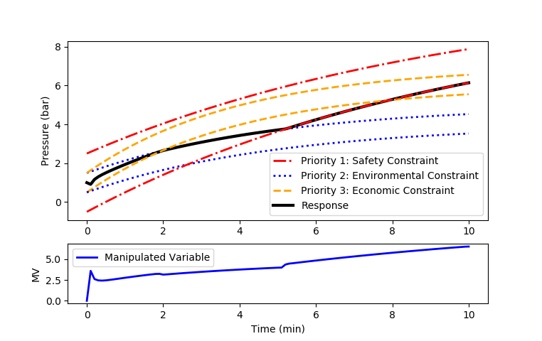
ax[0].plot(m.time,results['s.tr_hi'],'r-.',linewidth=2) ax[0].plot(m.time,results['y.tr_hi'],'b:',linewidth=2) ax[0].plot(m.time,results['z.tr_hi'],,color='orange',linewidth=2) ax[0].plot(m.time,results['z'],'k-',linewidth=3) ax[0].legend(['Priority 1: Safety Constraint', 'Priority 2: Environmental Constraint', 'Priority 3: Economic Constraint','Response'],loc=4) ax[0].plot(m.time,results['z.tr_lo'],,color='orange',linewidth=2) ax[0].plot(m.time,results['y.tr_lo'],'b:',linewidth=2) ax[0].plot(m.time,results['s.tr_lo'],'r-.',linewidth=2) ax[0].set_ylabel('Pressure (bar)')

ax[1].plot(m.time,u.value,'b-',linewidth=2) ax[1].legend(['Manipulated Variable']) ax[1].set_ylabel('MV') ax[1].set_xlabel('Time (min)')

plt.show() (:sourceend:) (:divend:)

(:html:) <iframe width="560" height="315" src="https://www.youtube.com/embed/JlMVZmGgjDY" frameborder="0" allowfullscreen></iframe> (:htmlend:)

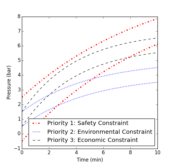
Many optimization problems have multiple competing objectives. These competing objectives are part of the trade-off that defines an optimal solution. Sometimes these competing objectives have separate priorities where one objective should be satisfied before another objective is even considered. This especially arises in model predictive control or other types of dynamic optimization problems. There are competing objectives with a ranked hierarchy. The highest level objectives are satisfied first followed by lower ranked objectives if there are additional degrees of freedom available. The l1-norm objective is a natural way to explicitly rank objectives and simultaneously optimize multiple priorities with a single optimization problem.

Exercise

Consider examples of safety, environmental, and economic constraints or objectives. Which are most important and why?

For the following multi-objective optimization problem, sketch a possible optimal trajectory.

Multiple Objectives

(:title Multi-Objective Optimization:) (:keywords multiple objectives, Python, MATLAB, Simulink, nonlinear control, model predictive control:) (:description Multiple objectives are simultaneously optimized to follow the highest priority objectives:)

Solution

Multi-Objective Model Predictive Control