Simulation of Dynamic Systems
Main.ModelSimulation History
Hide minor edits - Show changes to markup
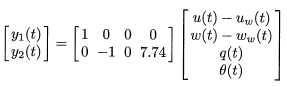
$$\begin{bmatrix} y_1(t) \\ y_2(t) \\ \end{bmatrix} = \begin{bmatrix} 1 & 0 & 0 & 0 \\ 0 & -1 & 0 & 7.74 \\ \end{bmatrix} \begin{bmatrix} u(t) - u_w(t) \\ w(t) - w_w(t) \\ q(t) \\ \theta(t) \\ \end{bmatrix}$$
$$\begin{bmatrix} y_1 \\ y_2 \\ \end{bmatrix} = \begin{bmatrix} 1 & 0 & 0 & 0 \\ 0 & -1 & 0 & 7.74 \\ \end{bmatrix} \begin{bmatrix} u - u_w \\ w - w_w \\ q \\ \theta \\ \end{bmatrix}$$
$$\begin{bmatrix} y_1(t) \\ y_2(t) \\ \end{bmatrix} = \begin{bmatrix} 1 & 0 & 0 & 0 \\ 0 & -1 & 0 & 7.74 \\ \end{bmatrix} \begin{bmatrix} u(t) - u_w(t) \\ w(t) - w_w(t) \\ q(t) \\ \theta(t) \\ \end{bmatrix}$$
from __future__ import division
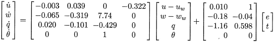
$$\begin{bmatrix} \dot{u} \\ \dot{w} \\ \dot{q} \\ \dot{\theta} \\ \end{bmatrix} = \begin{bmatrix} -0.003 & 0.039 & 0 & -0.322 \\ -0.065 & -0.319 & 7.74 & 0 \\ 0.020 & -0.101 & -0.429 & 0 \\ 0 & 0 & 1 & 0 \\ \end{bmatrix} \begin{bmatrix} u - u_w \\ w - w_w \\ q \\ \theta \\ \end{bmatrix} + \begin{bmatrix} 0.010 & 1 \\ -0.18 & -0.04 \\ -1.16 & 0.598 \\ 0 & 0 \\ \end{bmatrix} \begin{bmatrix} e \\ t \\ \end{bmatrix}$$
plt.plot(m.time,u[0],'b-',linewidth=2.0) plt.plot(m.time,u[1],'g:',linewidth=2.0)
plt.plot(m.time,u[0],'b-',lw=2.0) plt.plot(m.time,u[1],'g:',lw=2.0)
plt.plot(m.time,y[0],'r-',linewidth=2.0)
plt.plot(m.time,y[0],'r-',lw=2.0)
plt.plot(m.time,y[1],'r-',linewidth=2.0)
plt.plot(m.time,y[1],'r-',lw=2.0)
from gekko import SS
from gekko import GEKKO
m,x,y,u = SS(A,B,C)
m = GEKKO() x,y,u = m.state_space(A,B,C,D=None)
- get additional solution information (trajectories)
import json with open(m.path+'//results.json') as f:
results = json.load(f)
- get internal GEKKO variable names
air_speed = y[0].name climb_rate = y[1].name
plt.plot(m.time,u[0],'r-',linewidth=2.0) plt.plot(m.time,u[1],'k:',linewidth=2.0)
plt.plot(m.time,u[0],'b-',linewidth=2.0) plt.plot(m.time,u[1],'g:',linewidth=2.0)
plt.plot(m.time,y[0],'b:',linewidth=2.0)
- plt.plot(m.time,y[0].tr_hi,'k-')
- plt.plot(m.time,y[0].tr_lo,'k-')
plt.plot(m.time,y[0],'r-',linewidth=2.0) plt.plot(m.time,results[air_speed+'.tr_hi'],'k:') plt.plot(m.time,results[air_speed+'.tr_lo'],'k:')
plt.ylabel('Air Speed')
plt.plot(m.time,y[1],'g--',linewidth=2.0)
- plt.plot(m.time,y[1].tr_hi,'k-')
- plt.plot(m.time,y[1].tr_lo,'k-')
plt.plot(m.time,y[1],'r-',linewidth=2.0) plt.plot(m.time,results[climb_rate+'.tr_hi'],'k:') plt.plot(m.time,results[climb_rate+'.tr_lo'],'k:')
plt.ylabel('Climb Rate')
(:toggle hide gekko button show="Show GEKKO (Python) Code":) (:div id=gekko:) (:source lang=python:) from __future__ import division
from gekko import SS import numpy as np
- Linear model of a Boeing 747
- Level flight at 40,000 ft elevation
- Velocity at 774 ft/sec (0.80 Mach)
- States
- u - uw (ft/sec) - horizontal velocity - horizontal wind
- w - ww (ft/sec) - vertical velocity - vertical wind
- q (crad/sec) - angular velocity
- theta (crad) - angle from horizontal
- note: crad = 0.01 rad
- Inputs
- e - elevator
- t - throttle
- Outputs
- u - uw (ft/sec) - horizontal airspeed
- hdot = -w + u0 * theta with u0 = 774 ft/sec
A = np.array([[-.003, 0.039, 0, -0.322],
              [-0.065, -0.319, 7.74, 0],
              [0.020, -0.101, -0.429, 0],
              [0, 0, 1, 0]])
B = np.array([[0.01, 1],
              [-0.18, -0.04],
              [-1.16, 0.598],
              [0, 0]])
C = np.array([[1, 0, 0, 0],
[0, -1, 0, 7.74]])
- Build GEKKO State Space model
m,x,y,u = SS(A,B,C)
m.time = [0, 0.1, 0.2, 0.4, 1, 1.5, 2, 3, 4, 5, 6, 7, 8, 10, 12, 15] m.options.imode = 6 m.options.nodes = 3
- MV tuning
- lower and upper bounds for elevator pitch
- lower and upper bounds for thrust
- delta MV movement cost
for i in range(len(u)):
    u[i].lower = -5
    u[i].upper = 5
    u[i].dcost = 1
    u[i].status = 1
- CV tuning
- tau = first order time constant for trajectories
y[0].tau = 5 y[1].tau = 8
- tr_init = 0 (dead-band)
- = 1 (first order trajectory)
- = 2 (first order traj, re-center with each cycle)
y[0].tr_init = 2 y[1].tr_init = 2
- targets (dead-band needs upper and lower values)
- SPHI = upper set point
- SPLO = lower set point
y[0].sphi= -8.5 y[0].splo= -9.5 y[1].sphi= 5.4 y[1].splo= 4.6
y[0].status = 1 y[1].status = 1
m.solve()
- plot results
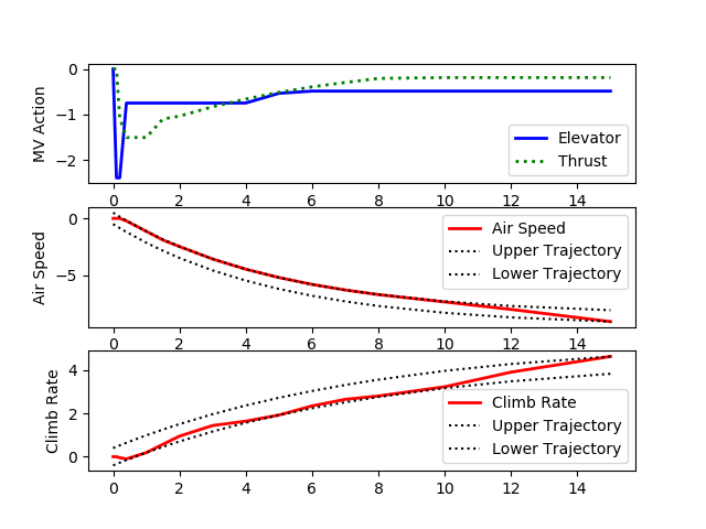
import matplotlib.pyplot as plt plt.figure(1) plt.subplot(311) plt.plot(m.time,u[0],'r-',linewidth=2.0) plt.plot(m.time,u[1],'k:',linewidth=2.0) plt.legend(['Elevator','Thrust']) plt.ylabel('MV Action')
plt.subplot(312) plt.plot(m.time,y[0],'b:',linewidth=2.0)
- plt.plot(m.time,y[0].tr_hi,'k-')
- plt.plot(m.time,y[0].tr_lo,'k-')
plt.legend(['Air Speed','Upper Trajectory','Lower Trajectory'])
plt.subplot(313) plt.plot(m.time,y[1],'g--',linewidth=2.0)
- plt.plot(m.time,y[1].tr_hi,'k-')
- plt.plot(m.time,y[1].tr_lo,'k-')
plt.legend(['Climb Rate','Upper Trajectory','Lower Trajectory'])
plt.show() (:sourceend:) (:divend:)
(:html:) <iframe width="560" height="315" src="https://www.youtube.com/embed/o_VlhBP4EfY?rel=0" frameborder="0" allowfullscreen></iframe> (:htmlend:)
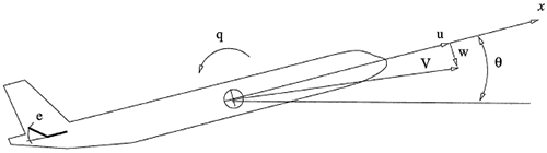
This exercise involves the simulation of a Boeing 747 airplane at cruising a cruising altitude of 40,000 ft. In this application1, a model of the process is desired to relate the elevator (e) and thrust (t) to the airspeed and climb rate. The model equations are shown below in state space form that relates elevator angle in centi-radians and thrust to four states including airspeed in the horizontal direction (u - u w), airspeed in the vertical direction (w - w w), rotation of the aircraft (q), and angle of the aircraft (theta).
This exercise involves the simulation of a Boeing 747 airplane at a cruising altitude of 40,000 ft. In this application1, a model of the process is desired to relate the elevator (e) and thrust (t) to the airspeed and climb rate. The model equations are shown below in state space form that relates elevator angle in centi-radians and thrust to four states including airspeed in the horizontal direction (u - u w), airspeed in the vertical direction (w - w w), rotation of the aircraft (q), and angle of the aircraft (theta).
This exercise involves the simulation of a Boeing 747 airplane at cruising a cruising altitude of 40,000 ft. In this application1, a model of the process is desired to relate the elevator (e) and thrust (t) to the airspeed and climb rate. The model equations are shown below in state space form that relates elevator angle in centi-radians and thrust to four states including airspeed in the horizontal direction (u'u w), airspeed in the vertical direction (w'w w), rotation of the aircraft (q), and angle of the aircraft (theta).
This exercise involves the simulation of a Boeing 747 airplane at cruising a cruising altitude of 40,000 ft. In this application1, a model of the process is desired to relate the elevator (e) and thrust (t) to the airspeed and climb rate. The model equations are shown below in state space form that relates elevator angle in centi-radians and thrust to four states including airspeed in the horizontal direction (u - u w), airspeed in the vertical direction (w - w w), rotation of the aircraft (q), and angle of the aircraft (theta).
This exercise involves the simulation of a Boeing 747 airplane at cruising a cruising altitude of 40,000 ft. In this application1, a model of the process is desired to relate the elevator (e) and thrust (t) to the airspeed and climb rate. The model equations are shown below in state space form that relates elevator angle in centi-radians and thrust to four states including airspeed in the horizontal direction (u'uw), airspeed in the vertical direction (w'ww), rotation of the aircraft (q), and angle of the aircraft (theta).
This exercise involves the simulation of a Boeing 747 airplane at cruising a cruising altitude of 40,000 ft. In this application1, a model of the process is desired to relate the elevator (e) and thrust (t) to the airspeed and climb rate. The model equations are shown below in state space form that relates elevator angle in centi-radians and thrust to four states including airspeed in the horizontal direction (u'u w), airspeed in the vertical direction (w'w w), rotation of the aircraft (q), and angle of the aircraft (theta).
The wind speeds are given in the horizontal (uw) and vertical (ww) directions with a nominal velocity of the aircraft of u0=774 ft/sec (0.8 Mach speed). The output y1 is the air speed and y2 is the climb rate.
The wind speeds are given in the horizontal (u w) and vertical (w w) directions with a nominal velocity of the aircraft of u0=774 ft/sec (0.8 Mach speed). The output y1 is the air speed and y2 is the climb rate.
The wind speeds are given in the horizontal (uw) and vertical (ww) directions with a nominal velocity of the aircraft of u0=774 ft/sec (0.8 Mach speed).
The wind speeds are given in the horizontal (uw) and vertical (ww) directions with a nominal velocity of the aircraft of u0=774 ft/sec (0.8 Mach speed). The output y1 is the air speed and y2 is the climb rate.
Simulate step responses of the aircraft with respect to the elevator angle and thrust. Design a model predictive controller to respond to set point changes in the air speed and climb rate of the aircraft. Explain the coordinated movement of the manipulated variables to achieve the desired set points of the controlled variables.
TBD

This exercise involves the simulation of a Boeing 747 airplane at cruising a cruising altitude of 40,000 ft. In this application1, a model of the process is desired to relate the elevator (e) and thrust (t) to the airspeed (u-uw) and climb rate (hrate).
This exercise involves the simulation of a Boeing 747 airplane at cruising a cruising altitude of 40,000 ft. In this application1, a model of the process is desired to relate the elevator (e) and thrust (t) to the airspeed and climb rate. The model equations are shown below in state space form that relates elevator angle in centi-radians and thrust to four states including airspeed in the horizontal direction (u'uw), airspeed in the vertical direction (w'ww), rotation of the aircraft (q), and angle of the aircraft (theta).
The wind speeds are given in the horizontal (uw) and vertical (ww) directions with a nominal velocity of the aircraft of u0=774 ft/sec (0.8 Mach speed).
flight_controls_747.png
flight_equations_747.png
Exercise
Exercise
flight_controls_747.png
This exercise involves the simulation of a Boeing 747 airplane at cruising a cruising altitude of 40,000 ft. In this application1, a model of the process is desired to relate the elevator (e) and thrust (t) to the airspeed (u-uw) and climb rate (hrate).
flight_equations_747.png
Solution
Solution
TBD
References
- Camacho, E.F. and Bordons, C., Model Predictive Control, 2nd Edition, Advanced Textbooks in Control and Signal Processing, Springer, 2004.
- Mass Balance
- Species Balance
- Energy Balance
- Funnel (Mass Balance)
- Mass Balance Solution
- Species Balance Solution
- Energy Balance Solution
- Funnel (Mass Balance) Solution
Exercise
Solution
Exercise
TBD
Solution
TBD
Develop and Solve Dynamic Equations
- Mass Balance
- Species Balance
- Energy Balance
- Funnel (Mass Balance)
Two numerical methods reviewed are sequential and simultaneous simulation techniques.
Sequential Simulation
Sequential simulation methods take successive time steps in the simulation horizon and often refine the size of each step to meet a specified error tolerance. Euler's method is the most basic method for sequential simulation while other methods generally offer improved accuracy and therefore allow larger step sizes.
<iframe width="560" height="315" src="https://www.youtube.com/embed/FE4GywqJmv0" frameborder="0" allowfullscreen></iframe>
<iframe width="560" height="315" src="https://www.youtube.com/embed/Oae-S5AzZCk" frameborder="0" allowfullscreen></iframe>
<iframe width="560" height="315" src="https://www.youtube.com/embed/0ah42LlU_3Y" frameborder="0" allowfullscreen></iframe>
<iframe width="560" height="315" src="https://www.youtube.com/embed/ynm7B0N0_Yw" frameborder="0" allowfullscreen></iframe>
(:html:) <iframe width="560" height="315" src="https://www.youtube.com/embed/AcNTTCjPCDg" frameborder="0" allowfullscreen></iframe> (:htmlend:)
(:html:) <iframe width="560" height="315" src="https://www.youtube.com/embed/diasyg2K_oU" frameborder="0" allowfullscreen></iframe> (:htmlend:)
Two numerical methods reviewed are sequential and simultaneous simulation techniques.
Sequential Simulation
Sequential simulation methods take successive time steps in the simulation horizon and often refine the size of each step to meet a specified error tolerance. Euler's method is the most basic method for sequential simulation while other methods generally offer improved accuracy and therefore allow larger step sizes.
(--video example with MATLAB / Python solvers)
(--include additional references--)
(--video example with APM MATLAB / APM Python solvers)
(--video example with APM MATLAB / APM Python solvers)
(video of numerical solution, APM MATLAB, APM Python, APMonitor - show how error changes with refined discretization)
(:html:) <iframe width="560" height="315" src="https://www.youtube.com/embed/pOXcOWMo5Hs" frameborder="0" allowfullscreen></iframe> (:htmlend:)
(:html:) <iframe width="560" height="315" src="https://www.youtube.com/embed/YvjG2LRNtKU" frameborder="0" allowfullscreen></iframe> (:htmlend:)
The DAE can be solved with a variety of numerical methods. Two numerical methods reviewed are sequential and simultaneous simulation techniques.
Sequential Simulation
The DAE can be solved with a variety of analytic or numeric methods. Analytic approaches are possible for simple systems such as systems with one or two equations. Numeric methods are used with more complicated systems but these methods have approximation errors that may deviate from the exact solution. A first step in model development is to draw a schematic, list the assumptions, and write the differential and algebraic equations that describe the system.
Develop and Solve Dynamic Equations
(:html:) <iframe width="560" height="315" src="https://www.youtube.com/embed/hje-dcn2cRw" frameborder="0" allowfullscreen></iframe> (:htmlend:)
(:html:) <iframe width="560" height="315" src="https://www.youtube.com/embed/FE4GywqJmv0" frameborder="0" allowfullscreen></iframe> (:htmlend:)
(:html:) <iframe width="560" height="315" src="https://www.youtube.com/embed/0ah42LlU_3Y" frameborder="0" allowfullscreen></iframe> (:htmlend:)
(:html:) <iframe width="560" height="315" src="https://www.youtube.com/embed/AcNTTCjPCDg" frameborder="0" allowfullscreen></iframe> (:htmlend:)
(:html:) <iframe width="560" height="315" src="https://www.youtube.com/embed/diasyg2K_oU" frameborder="0" allowfullscreen></iframe> (:htmlend:)
Two numerical methods reviewed are sequential and simultaneous simulation techniques.
Sequential Simulation
Simultaneous Simulation
Simultaneous Simulation
Exercise
Solution
Exercise
Solution
Sequential simulation methods take successive time steps in the simulation horizon and often refine the size of each step to meet a specified error tolerance. Euler's method is the most basic method for sequential simulation while other methods like the higher order Runga Kutta techniques generally offer improved accuracy and therefore allow larger step sizes.
Sequential simulation methods take successive time steps in the simulation horizon and often refine the size of each step to meet a specified error tolerance. Euler's method is the most basic method for sequential simulation while other methods generally offer improved accuracy and therefore allow larger step sizes.
(video of numerical solution, APM MATLAB, APM Python, APMonitor - show how error changes with refined discretization)
Nonlinear Modeling, Estimation and Predictive Control in APMonitor, Hedengren, J. D. and Asgharzadeh Shishavan, R., Powell, K.M., and Edgar, T.F., Computers and Chemical Engineering, Volume 70, pg. 133–148, 2014. Available at: https://dx.doi.org/10.1016/j.compchemeng.2014.04.013
(--include references--)
- Nonlinear Modeling, Estimation and Predictive Control in APMonitor, Hedengren, J. D. and Asgharzadeh Shishavan, R., Powell, K.M., and Edgar, T.F., Computers and Chemical Engineering, Volume 70, pg. 133–148, 2014. Available at: https://dx.doi.org/10.1016/j.compchemeng.2014.04.013
(--include additional references--)
Exercise
Solution
Nonlinear Modeling, Estimation and Predictive Control in APMonitor, Hedengren, J. D. and Asgharzadeh Shishavan, R., Powell, K.M., and Edgar, T.F., Computers and Chemical Engineering, Volume 70, pg. 133–148, 2014. Available at: https://dx.doi.org/10.1016/j.compchemeng.2014.04.013
Simulation of dynamic systems is the process of finding a numerical solution to a set of differential and algebraic equations (DAEs) with given initial conditions (x0). A mathematical expression of an Initial Value Problem (IVP) is shown as a set of
Simulation of dynamic systems is the process of finding a numerical solution to a set of differential and algebraic equations (DAEs) with given initial conditions (x0). A mathematical expression of an Initial Value Problem (IVP) is shown below.
Given x0 and p
Given x0 and p
The DAE can be solved with a variety of numerical methods. Two numerical methods reviewed are sequential and simultaneous simulation techniques.
Sequential Simulation
Sequential simulation methods take successive time steps in the simulation horizon and often refine the size of each step to meet a specified error tolerance. Euler's method is the most basic method for sequential simulation while other methods like the higher order Runga Kutta techniques generally offer improved accuracy and therefore allow larger step sizes.
(--video example with MATLAB / Python solvers)
Simultaneous Simulation
Simultaneous simulation methods are used to converge all of the state variable predictions together instead of one step at a time. Orthogonal collocation on finite elements is a popular method to convert the DAE into a Nonlinear Programming (NLP) problem for solution by efficient solvers.
 0 = f(x,p)
 0 < g(x,p)
 Given x0 and p
Further details on orthogonal collocation are provided at the following references.
(--include references--)
(--video example with APM MATLAB / APM Python solvers)
(--video example with APM MATLAB / APM Python solvers)
Simulation of dynamic systems is the process of finding a numerical solution to a set of differential and algebraic equations (DAEs) with given initial conditions (x0). A mathematical expression of an Initial Value Problem (IVP) is shown as a set of
 0 = f(dx/dt,x,p)
 0 < g(dx/dt,x,p)
 Given x0 and p
(:title Simulation of Dynamic Systems:) (:keywords simulation, sequential, simultaneous, ode solver, dae solver, modeling language, differential, algebraic, tutorial:) (:description Simmulation of Differential Algebraic Equations (DAEs) with use in dynamic simulation, estimation, and control:)