Estimation with Model Predictive Control
Main.EstimatorTypes History
Hide minor edits - Show changes to markup
Bias Update
Kalman Filter
Moving Horizon Estimation
The Kalman filter is an algorithm to estimate the state of a system in the presence of uncertain inputs. It is a recursive algorithm that uses a combination of previous system state, measurements and control inputs to estimate the current system state. The Kalman filter can be used for many applications such as object tracking, navigation and control system design.
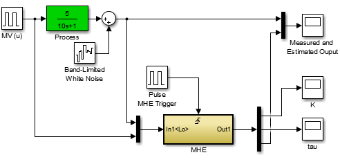
For this exercise, change the process model gain and time constant to unique values between 1 and 10. For example, the gain is 5.0 and the time constant is 10.0 in the Simulink model below as `\frac{5}{10s+1}`. There are three models in this exercise including the process, the estimator, and the controller. The first part of the exercise is to tune just the estimator. While an estimator can be well tuned to track measured values, it may be undesirable to have large parameter variations that are passed with each cycle to a model predictive controller.
For this exercise, change the process model gain and time constant to unique values between 1 and 10. For example, the gain is 5.0 and the time constant is 10.0 in the Simulink model below in Laplace form as `\frac{5}{10s+1}`. There are three models in this exercise including the process, the estimator, and the controller. The first part of the exercise is to tune just the estimator. While an estimator can be well tuned to track measured values, it may be undesirable to have large parameter variations that are passed with each cycle to a model predictive controller.
A linear, first order process is described by a gain K and time constant `\tau`. In transfer function form, this model is expressed as `\frac{K}{\tau \, s+1}` or in differential form as:
A linear, first order process is described by a gain K and time constant `\tau`. This model is expressed in differential form as:
For this exercise, change the model gain and time constant to unique values between 1 and 10. For example, the gain is 5.0 and the time constant is 10.0 in the model below. There are three models in this exercise including the process, the estimator, and the controller. The first part of the exercise is to tune the estimator.
For this exercise, change the process model gain and time constant to unique values between 1 and 10. For example, the gain is 5.0 and the time constant is 10.0 in the Simulink model below as `\frac{5}{10s+1}`. There are three models in this exercise including the process, the estimator, and the controller. The first part of the exercise is to tune just the estimator. While an estimator can be well tuned to track measured values, it may be undesirable to have large parameter variations that are passed with each cycle to a model predictive controller.
A linear, first order process is described by a gain K and time constant `\tau`. In transfer function form, this model is expressed as {`\frac{K}{\tau \, s+1}'' or in differential form as:
A linear, first order process is described by a gain K and time constant `\tau`. In transfer function form, this model is expressed as `\frac{K}{\tau \, s+1}` or in differential form as:
A linear, first order process is described by a gain K and time constant tau. In transfer function form, this model is expressed as K/(tau s+1) or in differential form as tau dy/dt = -y + K u. For this exercise, change the Simulink model gain and time constant to values between 1 and 10. For example, the gain is 5.0 and the time constant is 10.0 in the model below.
A linear, first order process is described by a gain K and time constant `\tau`. In transfer function form, this model is expressed as {`\frac{K}{\tau \, s+1}'' or in differential form as:
$$\tau \frac{dy}{dt} = -y + K \, u$$
For this exercise, change the model gain and time constant to unique values between 1 and 10. For example, the gain is 5.0 and the time constant is 10.0 in the model below. There are three models in this exercise including the process, the estimator, and the controller. The first part of the exercise is to tune the estimator.
Observe the estimator performance as new measurements arrive. Is the estimator able to reconstruct the unmeasured model parameters from the input and output data? Repeat the above exercise of changing the K and tau and run the MHE with MPC controller.
Observe the estimator performance as new measurements arrive. Is the estimator able to reconstruct the unmeasured model parameters from the input and output data?
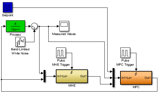
The second part is to tune the estimator for improved controller performance. When tuning an estimator for model predictive control performance, it is important to have more consistent parameter values that do not rapidly change cycle to cycle. Repeat the above exercise of changing the K and `\tau` and run the MHE with the MPC controller. Tune the estimator to give more consistent value of the unknown parameters and achieve better setpoint tracking.
Observe the controller performance as the estimator provides updated parameters (K and tau). Follow the flow of signals around the control loop to understand the specific inputs and outputs from each block. How does the controller perform if there is a mismatch between the estimated values of K and tau used in the controller and the process K and tau?
Observe the controller performance as the estimator provides updated parameters (K and `\tau`). Follow the flow of signals around the control loop to understand the specific inputs and outputs from each block. How does the controller perform if there is a mismatch between the estimated values of K and `\tau` used in the controller and the process K and `\tau`?
(:toggle hide gekko button show="Show GEKKO (Python) Code":)
(:toggle hide gekko button show="Show MHE GEKKO (Python) Code":)
(:toggle hide gekko2 button show="Show GEKKO (Python) Code":)
(:toggle hide gekko2 button show="Show MHE+MPC GEKKO (Python) Code":)
(:toggle hide gekko button show="Show GEKKO (Python) Code":) (:div id=gekko:) (:source lang=python:)
- Import packages
import numpy as np from random import random from gekko import GEKKO import matplotlib.pyplot as plt
- Process
p = GEKKO()
p.time = [0,.5]
- Parameters
p.u = p.MV() p.K = p.Param(value=1) #gain p.tau = p.Param(value=5) #time constant
- variable
p.y = p.SV() #measurement
- Equations
p.Equation(p.tau * p.y.dt() == -p.y + p.K * p.u)
- options
p.options.IMODE = 4
- MHE Model
m = GEKKO()
m.time = np.linspace(0,20,41) #0-20 by 0.5 -- discretization must match simulation
- Parameters
m.u = m.MV() #input m.K = m.FV(value=3, lb=1, ub=3) #gain m.tau = m.FV(value=4, lb=1, ub=10) #time constant
- Variables
m.y = m.CV() #measurement
- Equations
m.Equation(m.tau * m.y.dt() == -m.y + m.K*m.u)
- Options
m.options.IMODE = 5 #MHE m.options.EV_TYPE = 1 m.options.DIAGLEVEL = 0
- STATUS = 0, optimizer doesn't adjust value
- STATUS = 1, optimizer can adjust
m.u.STATUS = 0 m.K.STATUS = 1 m.tau.STATUS = 1 m.y.STATUS = 1
- FSTATUS = 0, no measurement
- FSTATUS = 1, measurement used to update model
m.u.FSTATUS = 1 m.K.FSTATUS = 0 m.tau.FSTATUS = 0 m.y.FSTATUS = 1
- DMAX = maximum movement each cycle
m.K.DMAX = 1 m.tau.DMAX = .1
- MEAS_GAP = dead-band for measurement / model mismatch
m.y.MEAS_GAP = 0.25
m.y.TR_INIT = 1
- problem configuration
- number of cycles
cycles = 50
- noise level
noise = 0.25
- run process, estimator and control for cycles
y_meas = np.empty(cycles) y_est = np.empty(cycles) k_est = np.empty(cycles) tau_est = np.empty(cycles) u_cont = np.empty(cycles) u = 2.0
- Create plot
plt.figure(figsize=(10,7)) plt.ion() plt.show()
for i in range(cycles):
    # change input (u)
    if i==10:
        u = 3.0
    elif i==20:
        u = 4.0
    elif i==30:
        u = 1.0
    elif i==40:
        u = 3.0
    u_cont[i] = u

    ## process simulator
    #load u value
    p.u.MEAS = u_cont[i]
    #simulate
    p.solve()
    #load output with white noise
    y_meas[i] = p.y.MODEL + (random()-0.5)*noise

    ## estimator
    #load input and measured output
    m.u.MEAS = u_cont[i]
    m.y.MEAS = y_meas[i]
    #optimize parameters
    m.solve()
    #store results
    y_est[i] = m.y.MODEL
    k_est[i] = m.K.NEWVAL
    tau_est[i] = m.tau.NEWVAL

    plt.clf()
    plt.subplot(4,1,1)
    plt.plot(y_meas[0:i])
    plt.plot(y_est[0:i])
    plt.legend(('meas','pred'))
    plt.ylabel('y')
    plt.subplot(4,1,2)
    plt.plot(np.ones(i)*p.K.value[0])
    plt.plot(k_est[0:i])
    plt.legend(('actual','pred'))
    plt.ylabel('k')
    plt.subplot(4,1,3)
    plt.plot(np.ones(i)*p.tau.value[0])
    plt.plot(tau_est[0:i])
    plt.legend(('actual','pred'))
    plt.ylabel('tau')
    plt.subplot(4,1,4)
    plt.plot(u_cont[0:i])
    plt.legend('u')
    plt.draw()
    plt.pause(0.05)
(:sourceend:) (:divend:)
(:toggle hide gekko2 button show="Show GEKKO (Python) Code":) (:div id=gekko2:) (:source lang=python:)
- Import packages
import numpy as np from random import random from gekko import GEKKO import matplotlib.pyplot as plt
- Process
p = GEKKO()
p.time = [0,.5]
- Parameters
p.u = p.MV() p.K = p.Param(value=1) #gain p.tau = p.Param(value=5) #time constant
- variable
p.y = p.SV() #measurement
- Equations
p.Equation(p.tau * p.y.dt() == -p.y + p.K * p.u)
- options
p.options.IMODE = 4
- MHE Model
m = GEKKO()
m.time = np.linspace(0,20,41) #0-20 by 0.5 -- discretization must match simulation
- Parameters
m.u = m.MV() #input m.K = m.FV(value=3, lb=1, ub=3) #gain m.tau = m.FV(value=4, lb=1, ub=10) #time constant
- Variables
m.y = m.CV() #measurement
- Equations
m.Equation(m.tau * m.y.dt() == -m.y + m.K*m.u)
- Options
m.options.IMODE = 5 #MHE m.options.EV_TYPE = 1 m.options.DIAGLEVEL = 0
- STATUS = 0, optimizer doesn't adjust value
- STATUS = 1, optimizer can adjust
m.u.STATUS = 0 m.K.STATUS = 1 m.tau.STATUS = 1 m.y.STATUS = 1
- FSTATUS = 0, no measurement
- FSTATUS = 1, measurement used to update model
m.u.FSTATUS = 1 m.K.FSTATUS = 0 m.tau.FSTATUS = 0 m.y.FSTATUS = 1
- DMAX = maximum movement each cycle
m.K.DMAX = 1 m.tau.DMAX = .1
- MEAS_GAP = dead-band for measurement / model mismatch
m.y.MEAS_GAP = 0.25
m.y.TR_INIT = 1
- MHE Model
c = GEKKO()
c.time = np.linspace(0,5,11) #0-5 by 0.5 -- discretization must match simulation
- Parameters
c.u = c.MV(lb=-10,ub=10) #input c.K = c.FV(value=10, lb=1, ub=3) #gain c.tau = c.FV(value=1, lb=1, ub=10) #time constant
- Variables
c.y = c.CV() #measurement
- Equations
c.Equation(c.tau * c.y.dt() == -c.y + c.u * c.K)
- Options
c.options.IMODE = 6 #MPC c.options.CV_TYPE = 1
- STATUS = 0, optimizer doesn't adjust value
- STATUS = 1, optimizer can adjust
c.u.STATUS = 1 c.K.STATUS = 0 c.tau.STATUS = 0 c.y.STATUS = 1
- FSTATUS = 0, no measurement
- FSTATUS = 1, measurement used to update model
c.u.FSTATUS = 0 c.K.FSTATUS = 1 c.tau.FSTATUS = 1 c.y.FSTATUS = 1
- DMAX = maximum movement each cycle
c.u.DCOST = .1
- y setpoint
- if CV_TYPE = 1, use SPHI and SPLO
sp = 3.0 c.y.SPHI = sp + 0.1 c.y.SPLO = sp - 0.1
- if CV_TYPE = 2, use SP
- c.y.SP = 3
c.y.TR_INIT = 0
- problem configuration
- number of cycles
cycles = 100
- noise level
noise = 0.25
- run process, estimator and control for cycles
y_meas = np.empty(cycles) y_est = np.empty(cycles) k_est = np.empty(cycles) tau_est = np.empty(cycles) u_cont = np.empty(cycles) sp_store = np.empty(cycles)
- Create plot
plt.figure(figsize=(10,7)) plt.ion() plt.show()
for i in range(cycles):
    # set point changes
    if i==20:
        sp = 5.0
    elif i==40:
        sp = 2.0
    elif i==60:
        sp = 4.0
    elif i==80:
        sp = 3.0
    c.y.SPHI = sp + 0.1
    c.y.SPLO = sp - 0.1
    sp_store[i] = sp

    ## controller
    #load
    c.tau.MEAS = m.tau.NEWVAL
    c.K.MEAS = m.K.NEWVAL
    if p.options.SOLVESTATUS == 1:
        c.y.MEAS = p.y.MODEL
    #change setpoint at time 25
    if i == 25:
        c.y.SPHI = 6.1
        c.y.SPLO = 5.9
    c.solve()
    u_cont[i] = c.u.NEWVAL

    ## process simulator
    #load control move
    p.u.MEAS = u_cont[i]
    #simulate
    p.solve()
    #load output with white noise
    y_meas[i] = p.y.MODEL + (random()-0.5)*noise

    ## estimator
    #load input and measured output
    m.u.MEAS = u_cont[i]
    m.y.MEAS = y_meas[i]
    #optimize parameters
    m.solve()
    #store results
    y_est[i] = m.y.MODEL
    k_est[i] = m.K.NEWVAL
    tau_est[i] = m.tau.NEWVAL

    plt.clf()
    plt.subplot(4,1,1)
    plt.plot(y_meas[0:i])
    plt.plot(y_est[0:i])
    plt.plot(sp_store[0:i])
    plt.legend(('meas','pred','setpoint'))
    plt.ylabel('y')
    plt.subplot(4,1,2)
    plt.plot(np.ones(i)*p.K.value[0])
    plt.plot(k_est[0:i])
    plt.legend(('actual','pred'))
    plt.ylabel('k')
    plt.subplot(4,1,3)
    plt.plot(np.ones(i)*p.tau.value[0])
    plt.plot(tau_est[0:i])
    plt.legend(('actual','pred'))
    plt.ylabel('tau')
    plt.subplot(4,1,4)
    plt.plot(u_cont[0:i])
    plt.legend('u')
    plt.draw()
    plt.pause(0.05)
(:sourceend:) (:divend:)
(:title Estimation Introduction: Bias Update, Kalman Filter, and MHE:)
(:title Estimation with Model Predictive Control:)
Objective: Implement MHE with an without Model Predictive Control (MPC). Understand the difference between tracking performance (agreement between model and measured values) and predictive performance (model parameters that predict into the future).
Objective: Implement MHE with an without Model Predictive Control (MPC). Describe the difference between tracking performance (agreement between model and measured values) and predictive performance (model parameters that predict into the future). Tune the estimator to improve control performance. Show how overly aggressive tracking performance may degrade the control performance even though the estimator performance (difference between measured and modeled output) is acceptable. An overly aggressive estimator may give different parameter values (K and tau) for each cycle.

Kalman filtering produces estimates of variables and parameters from data and Bayesian model predictions. The data may include inaccuracies such as noise (random fluctuations), outliers, or other inaccuracies. The Kalman filter is a recursive algorithm where additional measurements are used to update states (x) and an uncertainty description as a covariance matrix (P).
Kalman filtering produces estimates of variables and parameters from data and Bayesian model predictions. The data may include inaccuracies such as noise (random fluctuations), outliers, or other inaccuracies. The Kalman filter is a recursive algorithm where additional measurements are used to update states (x) and an uncertainty description as a covariance matrix (P).
(:html:) <iframe width="560" height="315" src="https://www.youtube.com/embed/KdGAfGRZSbs?rel=0" frameborder="0" allowfullscreen></iframe> (:htmlend:)
(:title Estimation: Bias and Kalman Filters:)
(:title Estimation Introduction: Bias Update, Kalman Filter, and MHE:)
Moving horizon estimation (MHE) is an optimization approach for predicting states and parameters. Model predictions are matched to a horizon of prior measurements by adjusting parameters and the initial conditions of the model.
A linear, first order process is described by a gain K and time constant tau. In transfer function form, this model is expressed as K/(tau s+1) or in differential form as tau dy/dt = -y + K u. For this exercise, change the Simulink model gain and time constant to values between 1 and 10. For example, the gain is 5.0 and the time constant is to 10.0 in the model below.
A linear, first order process is described by a gain K and time constant tau. In transfer function form, this model is expressed as K/(tau s+1) or in differential form as tau dy/dt = -y + K u. For this exercise, change the Simulink model gain and time constant to values between 1 and 10. For example, the gain is 5.0 and the time constant is 10.0 in the model below.
A linear, first order process is described by a gain K and time constant tau. In transfer function form, this model is expressed as K/(tau s+1) or in differential form as tau dy/dt = -y + K u. For this exercise, change the Simulink model gain and time constant to values between 1 and 10. For example, change the gain to 6.5 and the time constant to 2.0.
A linear, first order process is described by a gain K and time constant tau. In transfer function form, this model is expressed as K/(tau s+1) or in differential form as tau dy/dt = -y + K u. For this exercise, change the Simulink model gain and time constant to values between 1 and 10. For example, the gain is 5.0 and the time constant is to 10.0 in the model below.
A linear, first order process is described by a gain K and time constant tau. In transfer function form, this model is expressed as K/(tau s+1) or in differential form as tau dy/dt = -y + K u. For this exercise, change the Simulink model gain and time constant to values between 1 and 10.
A linear, first order process is described by a gain K and time constant tau. In transfer function form, this model is expressed as K/(tau s+1) or in differential form as tau dy/dt = -y + K u. For this exercise, change the Simulink model gain and time constant to values between 1 and 10. For example, change the gain to 6.5 and the time constant to 2.0.
The extended Kalman filter (EKF) is the same as the Kalman filter but in applications that have a nonlinear model. The model is relinearized at every new prediction step to extend the linear methods for nonlinear cases. The unscented Kalman filter (UKF) shows improved performance for systems that are highly nonlinear or have non-uniform probability distributions for the estimates. UKF uses sigma points (sample points that are selected to represent the uncertainty of the states) that are propagated forward in time with the use of simulation. Points that are closest to the measured values are retained while points that are beyond a tolerance value are removed. Additional sigma points are added at each sampling instance to maintain a population of points that represent a collection of potential state values.
The extended Kalman filter (EKF) is the same as the Kalman filter but in applications that have a nonlinear model. The model is relinearized at every new prediction step to extend the linear methods for nonlinear cases. The unscented Kalman filter (UKF) shows improved performance for systems that are highly nonlinear or have non-uniform probability distributions for the estimates. UKF uses sigma points (sample points that are selected to represent the uncertainty of the states) that are propagated forward in time with the use of simulation. Points that are closest to the measured values are retained while points that are beyond a tolerance value are removed. Additional sigma points are added at each sampling instance to maintain a population of points that represent a collection of potential state values.
Exercise
Objective: Implement MHE with an without Model Predictive Control (MPC). Understand the difference between tracking performance (agreement between model and measured values) and predictive performance (model parameters that predict into the future).
A linear, first order process is described by a gain K and time constant tau. In transfer function form, this model is expressed as K/(tau s+1) or in differential form as tau dy/dt = -y + K u. For this exercise, change the Simulink model gain and time constant to values between 1 and 10.
Observe the estimator performance as new measurements arrive. Is the estimator able to reconstruct the unmeasured model parameters from the input and output data? Repeat the above exercise of changing the K and tau and run the MHE with MPC controller.
Observe the controller performance as the estimator provides updated parameters (K and tau). Follow the flow of signals around the control loop to understand the specific inputs and outputs from each block. How does the controller perform if there is a mismatch between the estimated values of K and tau used in the controller and the process K and tau?
Solution
(:title Estimation with Biasing and Kalman Filtering:)
(:title Estimation: Bias and Kalman Filters:)
(:title Dynamic Estimation: Biasing, EKF, UKF:)
(:title Estimation with Biasing and Kalman Filtering:)
Kalman filtering produces estimates of variables and parameters from data and Bayesian model predictions. The data may include inaccuracies such as noise (random fluctuations), outliers, or other inaccuracies. The Kalman filter is a recursive algorithm where additional measurements are used to update states (x) and an uncertainty description as a covariance matrix (P).
Kalman filtering produces estimates of variables and parameters from data and Bayesian model predictions. The data may include inaccuracies such as noise (random fluctuations), outliers, or other inaccuracies. The Kalman filter is a recursive algorithm where additional measurements are used to update states (x) and an uncertainty description as a covariance matrix (P).
The extended Kalman filter (EKF) is the same as the Kalman filter but in applications that have a nonlinear model. The model is relinearized at every new prediction step to extend the linear methods for nonlinear cases. The unscented Kalman filter (UKF) shows improved performance for systems that are highly nonlinear or have non-uniform probability distributions for the estimates. UKF uses sigma points (sample points that are selected to represent the uncertainty of the states) that are propagated forward in time with the use of simulation. Points that are closest to the measured values are retained while points that are beyond a tolerance value are removed. Additional sigma points are added at each sampling instance to maintain a population of points that represent a collection of potential state values.
(:title Dynamic Estimation: Biasing, EKF, UKF:) (:keywords Kalman filter, unscented Kalman filter, extended Kalman filter, dynamic data, validation, estimation, simulation, modeling language, differential, algebraic, tutorial:) (:description Dynamic estimation with simple biasing, extended Kalman filter, or unscented Kalman filter:)
Simple biasing, Kalman filters, and Moving Horizon Estimation (MHE) are all approaches to align dynamic data with model predictions. Each method has particular advantages and disadvantages with a main trade-off being algorithmic complexity versus quality of the solution.
Biasing is a method to adjust output values with either an additive or multiplicative term. The additive or multiplicative bias is increased or decreased depending on the current difference between model prediction and measured value. This is the most basic form of model updates and it is prevalent in industrial base control and advanced control applications.
Kalman filtering produces estimates of variables and parameters from data and Bayesian model predictions. The data may include inaccuracies such as noise (random fluctuations), outliers, or other inaccuracies. The Kalman filter is a recursive algorithm where additional measurements are used to update states (x) and an uncertainty description as a covariance matrix (P).