Dynamic Optimization

plt.plot(m.time,x1.value,'k:',lw=2,label=r'$x_1$') plt.plot(m.time,x2.value,'b-',lw=2,label=r'$x_2$') plt.plot(m.time,u.value,'r--',lw=2,label=r'$u$')

plt.plot(m.time,x1.value,'k:',lw=2,label=r'$x_1$') plt.plot(m.time,x2.value,'b-',lw=2,label=r'$x_2$') plt.plot(m.time,u.value,'r--',lw=2,label=r'$u$')

plt.plot(m.time,u,'r-',lw=2,label=r'$u$')

plt.plot(m.time,x1.value,'r--',lw=2,label=r'$x_1$') plt.plot(m.time,x2.value,'g:',lw=2,label=r'$x_2$') plt.plot(m.time,x3.value,'k-',lw=2,label=r'$x_3$') plt.plot(m.time,x4.value,'b-',lw=2,label=r'$x_4$')

plt.plot(m.time,x1.value,'k:',lw=2,label=r'$x_1$') plt.plot(m.time,x2.value,'b-',lw=2,label=r'$x_2$') plt.plot(m.time,u.value,'r--',lw=2,label=r'$u$')

plt.plot(m.time,x1.value,'k:',lw=2,label=r'$x_1$') plt.plot(m.time,x2.value,'b-',lw=2,label=r'$x_2$')

plt.plot(m.time,T.value,'r--',lw=2,label=r'$T$')

plt.plot(m.time,x1.value,'k:',lw=2,label=r'$x_1$') plt.plot(m.time,x2.value,'b-',lw=2,label=r'$x_2$')

plt.plot(m.time,u.value,'r-',lw=2,label=r'$u$')

(:title Optimal Control Benchmark Problems:)

Objective: Solve the dynamic optimization benchmark problems² and more dynamic optimization benchmark problems. Complete the 9 exercises as shown in the Jupyter Notebook link below. For each problem, create a program to optimize and display the results. Estimated Time (each): 10-30 minutes

Objective: Solve the dynamic optimization benchmark problems² and MoreDynamicOptimizationBenchmarks. For each problem, create a program to optimize and display the results. Estimated Time (each): 30 minutes

Dynamic Optimization Benchmarks on GitHub or on Google Colab.

$$\frac{dx_4}{dt}=x_1^2+x_2^2+0.005 \left(x_2 + 16 \, t -8 -0.1x_3\,u^2\right)^2$$

(:title Optimal Control Problems:) (:keywords nonlinear control, optimal control, dynamic optimization, engineering optimization, MATLAB, Python, GEKKO, differential, algebraic, modeling language, university course:) (:description Optimal control problems solved with Dynamic Optimization in MATLAB, Excel, and Python.:)

(:html:) <iframe width="560" height="315" src="https://www.youtube.com/embed/r42PEsh5Nxg" frameborder="0" allow="autoplay; encrypted-media" allowfullscreen></iframe> (:htmlend:)

(:html:) <iframe width="560" height="315" src="https://www.youtube.com/embed/gptRJ5x7Ybs" frameborder="0" allow="autoplay; encrypted-media" allowfullscreen></iframe> (:htmlend:)

(:html:) <iframe width="560" height="315" src="https://www.youtube.com/embed/mdefRrGarP0" frameborder="0" allow="autoplay; encrypted-media" allowfullscreen></iframe> (:htmlend:)

(:html:) <iframe width="560" height="315" src="https://www.youtube.com/embed/mdefRrGarP0" frameborder="0" allow="autoplay; encrypted-media" allowfullscreen></iframe> (:htmlend:)

(:html:) <iframe width="560" height="315" src="https://www.youtube.com/embed/mdefRrGarP0" frameborder="0" allow="autoplay; encrypted-media" allowfullscreen></iframe> (:htmlend:)

(:html:) <iframe width="560" height="315" src="https://www.youtube.com/embed/dxC__nDnmCY" frameborder="0" allow="autoplay; encrypted-media" allowfullscreen></iframe> (:htmlend:)

import numpy as np import matplotlib.pyplot as plt from gekko import GEKKO

m = GEKKO()

nt = 101 m.time = np.linspace(0,12,nt)

1. Parameters

u = m.MV(value=1,ub=1,lb=0) u.STATUS = 1 u.DCOST = 0

1. Variables

x1 = m.Var(value=1) x2 = m.Var(value=0)

p = np.zeros(nt) p[-1] = 1.0 final = m.Param(value=p)

1. Equations

m.Equation(x1.dt()==u*(10*x2-x1)) m.Equation(x2.dt()==-u*(10*x2-x1)-(1-u)*x2)

1. Objective Function

m.Obj(-final*(1-x1-x2))

m.options.IMODE = 6 m.solve()

print('Objective: ' + str(1-x1[-1]-x2[-1]))

plt.figure(1)

plt.subplot(2,1,1) plt.plot(m.time,x1.value,'k:',LineWidth=2,label=r'$x_1$') plt.plot(m.time,x2.value,'b-',LineWidth=2,label=r'$x_2$') plt.ylabel('Value') plt.legend(loc='best')

plt.subplot(2,1,2) plt.plot(m.time,u.value,'r-',LineWidth=2,label=r'$u$') plt.legend(loc='best') plt.xlabel('Time') plt.ylabel('Value')

plt.show()

import numpy as np import matplotlib.pyplot as plt from gekko import GEKKO

m = GEKKO()

nt = 101 m.time = np.linspace(0,1,nt)

1. Parameters

T = m.MV(value=362,ub=398,lb=298) T.STATUS = 1 T.DCOST = 0

1. Variables

x1 = m.Var(value=1) x2 = m.Var(value=0)

p = np.zeros(nt) p[-1] = 1.0 final = m.Param(value=p)

1. Intermediates

k1 = m.Intermediate(4000*m.exp(-2500/T)) k2 = m.Intermediate(6.2e5*m.exp(-5000/T))

1. Equations

m.Equation(x1.dt()==-k1*x1**2) m.Equation(x2.dt()==k1*x1**2 - k2*x2)

1. Objective Function

m.Obj(-x2*final)

m.options.IMODE = 6 m.solve()

print('Objective: ' + str(x2[-1]))

plt.figure(1)

plt.subplot(2,1,1) plt.plot(m.time,x1.value,'k:',LineWidth=2,label=r'$x_1$') plt.plot(m.time,x2.value,'b-',LineWidth=2,label=r'$x_2$') plt.ylabel('Value') plt.legend(loc='best')

plt.subplot(2,1,2) plt.plot(m.time,T.value,'r--',LineWidth=2,label=r'$T$') plt.legend(loc='best') plt.xlabel('Time') plt.ylabel('Value')

plt.show()

import numpy as np import matplotlib.pyplot as plt from gekko import GEKKO

m = GEKKO()

nt = 101 m.time = np.linspace(0,1,nt)

1. Parameters

u = m.MV(value=1,ub=5,lb=0) u.STATUS = 1

1. Variables

x1 = m.Var(value=1) x2 = m.Var(value=0)

p = np.zeros(nt) p[-1] = 1.0 final = m.Param(value=p)

1. Equations

m.Equation(x1.dt()==-(u+0.5*u**2)*x1) m.Equation(x2.dt()==u*x1)

1. Objective Function

m.Obj(-x2*final)

m.options.IMODE = 6 m.solve()

print('Objective: ' + str(x2[-1]))

plt.figure(1) plt.plot(m.time,x1.value,'k:',LineWidth=2,label=r'$x_1$') plt.plot(m.time,x2.value,'b-',LineWidth=2,label=r'$x_2$') plt.plot(m.time,u.value,'r--',LineWidth=2,label=r'$u$') plt.legend(loc='best') plt.xlabel('Time') plt.ylabel('Value') plt.show()

$$\max_{T(t)} x_2 \left( t_f \right)$$

$$\max_{u(t)} x_2 \left( t_f \right)$$

plt.plot(m.time,x1.value,'k:',LineWidth=2,label=r'$x_1$') plt.plot(m.time,x2.value,'b-',LineWidth=2,label=r'$x_2$') plt.plot(m.time,u.value,'r--',LineWidth=2,label=r'$u$')

plt.plot(m.time,x1.value,'k:',LineWidth=2,label=r'$x_1$') plt.plot(m.time,x2.value,'b-',LineWidth=2,label=r'$x_2$') plt.plot(m.time,u.value,'r--',LineWidth=2,label=r'$u$')

plt.plot(m.time,x1.value,'r--',LineWidth=2,label=r'$x_1$') plt.plot(m.time,x2.value,'g:',LineWidth=2,label=r'$x_2$') plt.plot(m.time,x3.value,'k-',LineWidth=2,label=r'$x_3$') plt.plot(m.time,x4.value,'b-',LineWidth=2,label=r'$x_4$')

Solutions to Benchmarks 1a and 1b

(:toggle hide solution1 button show="Show Solutions for Problem 1a and 1b":) (:div id=solution1:)

(:divend:)

(:html:) <iframe width="560" height="315" src="https://www.youtube.com/embed/WHnIfKUfjQY" frameborder="0" allow="autoplay; encrypted-media" allowfullscreen></iframe> (:htmlend:)

$$\max_{u(t)} \left(1 - x_1 \left( t_f \right) - x_2 \left( t_f \right) \right)$$

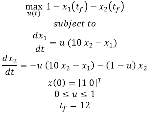
$$\min_{u(t)} 1 - x_1 \left( t_f \right) - x_2 \left( t_f \right)$$ $$\mathrm{subject \; to}$$ $$\frac{dx_1}{dt}=u \left(10 \, x_2 - x_1 \right)$$ $$\frac{dx_2}{dt}=-u \left(10 \, x_2 - x_1 \right)-\left(1-u\right) x_2$$ $$x(0) = [1 \; 0]^T$$ $$0 \le u \le 1$$ $$t_f=12$$

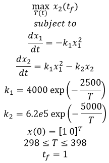
$$\min_{T(t)} x_2 \left( t_f \right)$$ $$\mathrm{subject \; to}$$ $$\frac{dx_1}{dt}=-k_1 \, x_1^2$$ $$\frac{dx_2}{dt}=k_1 \, x_1^2 - k_2 \, x_2$$ $$k_1 = 4000 \, \exp{\left(-\frac{2500}{T}\right)}$$ $$k_2 = 6.2e5 \, \exp{\left(-\frac{5000}{T}\right)}$$ $$x(0) = [1 \; 0]^T$$ $$298 \le T \le 398$$ $$t_f=1$$

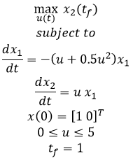
$$\min_{u(t)} x_2 \left( t_f \right)$$ $$\mathrm{subject \; to}$$ $$\frac{dx_1}{dt}=-\left(u+0.5u^2\right) x_1$$ $$\frac{dx_2}{dt}=u \, x_1$$ $$x(0) = [1 \; 0]^T$$ $$0 \le u \le 5$$ $$t_f=1$$

import numpy as np import matplotlib.pyplot as plt from gekko import GEKKO

m = GEKKO()

nt = 101 m.time = np.linspace(0,1,nt)

1. Parameters

u = m.MV(value=9,lb=-4,ub=10) u.STATUS = 1 u.DCOST = 0

1. Variables

t = m.Var(value=0) x1 = m.Var(value=0) x2 = m.Var(value=-1) x3 = m.Var(value=-np.sqrt(5)) x4 = m.Var(value=0)

p = np.zeros(nt) p[-1] = 1.0 final = m.Param(value=p)

1. Equations

m.Equation(t.dt()==1) m.Equation(x1.dt()==x2) m.Equation(x2.dt()==-x3*u+16*t-8) m.Equation(x3.dt()==u) m.Equation(x4.dt()==x1**2+x2**2 +0.005*(x2+16*t-8-0.1*x3*(u**2))**2)

1. Objective Function

m.Obj(x4*final)

m.options.IMODE = 6 m.options.NODES = 4 m.options.MV_TYPE = 1 m.options.SOLVER = 3 m.solve()

print(m.path)

print('Objective = min x4(tf): ' + str(x4[-1]))

plt.figure(1) plt.subplot(2,1,1) plt.plot(m.time,u,'r-',LineWidth=2,label=r'$u$') plt.legend(loc='best') plt.subplot(2,1,2) plt.plot(m.time,x1,'r--',LineWidth=2,label=r'$x_1$') plt.plot(m.time,x2,'g:',LineWidth=2,label=r'$x_2$') plt.plot(m.time,x3,'k-',LineWidth=2,label=r'$x_3$') plt.plot(m.time,x4,'b-',LineWidth=2,label=r'$x_4$') plt.legend(loc='best') plt.xlabel('Time') plt.ylabel('Value') plt.show()

nt = 101

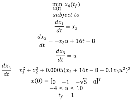
$$\min_{u(t)} x_4 \left( t_f \right)$$ $$\mathrm{subject \; to}$$ $$\frac{dx_1}{dt}=x_2$$ $$\frac{dx_2}{dt}=-x_3 \, u + 16 \, t - 8$$ $$\frac{dx_3}{dt}=u$$ $$\frac{dx_4}{dt}=x_1^2+x_2^2+0.0005 \left(x_2 + 16 \, t -8 -0.1x_3\,u^2\right)^2$$ $$x(0) = [0 \; -1 \; -\sqrt{5} \; 0]^T$$ $$-4 \le u \le 10$$ $$t_f=1$$

$$x(0) = [1 \; 0]^T$$

Example 1b

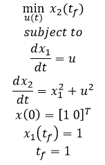
• Nonlinear, unconstrained, minimize final state with terminal constraint

$$\min_{u(t)} x_2 \left( t_f \right)$$ $$\mathrm{subject \; to}$$ $$\frac{dx_1}{dt}=u$$ $$\frac{dx_2}{dt}=x_1^2 + u^2$$ $$x(0) = [1 \; 0]^T$$ $$x_1 \left( t_f \right)=1$$ $$t_f=1$$

Solution to Benchmarks 1a and 1b

Dynamic Optimization Benchmark 1a and 1b in MATLAB and Python

(:html:) <iframe width="560" height="315" src="https://www.youtube.com/embed/mmCFF3-6sGg" frameborder="0" allowfullscreen></iframe> (:htmlend:)

(:toggle hide gekko1a button show="Show GEKKO (Python) Code for 1a":)

(:toggle hide gekko1b button show="Show GEKKO (Python) Code for 1b":) (:div id=gekko1b:) (:source lang=python:) import numpy as np import matplotlib.pyplot as plt from gekko import GEKKO

m = GEKKO()

nt = 101 m.time = np.linspace(0,1,nt)

1. Variables

x1 = m.Var(value=1) x2 = m.Var(value=0) u = m.Var(value=-0.48)

p = np.zeros(nt) p[-1] = 1.0 final = m.Param(value=p)

1. Equations

m.Equation(x1.dt()==u) m.Equation(x2.dt()==x1**2 + u**2) m.Equation(final*(x1-1)==0)

1. Objective Function

m.Obj(x2*final)

m.options.IMODE = 6 m.solve()

plt.figure(1) plt.plot(m.time,x1,'k:',LineWidth=2,label=r'$x_1$') plt.plot(m.time,x2,'b-',LineWidth=2,label=r'$x_2$') plt.plot(m.time,u,'r--',LineWidth=2,label=r'$u$') plt.legend(loc='best') plt.xlabel('Time') plt.ylabel('Value') plt.show() (:sourceend:) (:divend:)

(:toggle hide gekko2 button show="Show GEKKO (Python) Code":) (:div id=gekko2:) (:source lang=python:)

1. Show source

(:sourceend:) (:divend:)

(:toggle hide gekko3 button show="Show GEKKO (Python) Code":) (:div id=gekko3:) (:source lang=python:)

1. Show source

(:sourceend:) (:divend:)

(:toggle hide gekko4 button show="Show GEKKO (Python) Code":) (:div id=gekko4:) (:source lang=python:)

1. Show source

(:sourceend:) (:divend:)

(:toggle hide gekko5 button show="Show GEKKO (Python) Code":) (:div id=gekko5:) (:source lang=python:)

1. Show source

(:sourceend:) (:divend:)

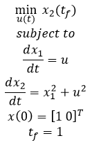
$$\min_{u(t)} x_2 \left( t_f \right)$$ $$\mathrm{subject \; to}$$ $$\frac{dx_1}{dt}=u$$ $$\frac{dx_2}{dt}=x_1^2 + u^2$$ $$x(0) = [1 0]^T$$ $$t_f=1$$

Objective: Set up and solve three of the five dynamic optimization benchmark problems². Create a program to optimize and display the results. Estimated Time (each): 30 minutes

(:toggle hide gekko1a button show="Show GEKKO (Python) Code":) (:div id=gekko1a:) (:source lang=python:) import numpy as np import matplotlib.pyplot as plt from gekko import GEKKO

m = GEKKO()

nt = 501 m.time = np.linspace(0,1,nt)

1. Variables

x1 = m.Var(value=1) x2 = m.Var(value=0) u = m.Var(value=-0.75)

p = np.zeros(nt) p[-1] = 1.0 final = m.Param(value=p)

1. Equations

m.Equation(x1.dt()==u) m.Equation(x2.dt()==x1**2 + u**2)

1. Objective Function

m.Obj(x2*final)

m.options.IMODE = 6 m.solve()

plt.figure(1) plt.plot(m.time,x1,'k:',LineWidth=2,label=r'$x_1$') plt.plot(m.time,x2,'b-',LineWidth=2,label=r'$x_2$') plt.plot(m.time,u,'r--',LineWidth=2,label=r'$u$') plt.legend(loc='best') plt.xlabel('Time') plt.ylabel('Value') plt.show() (:sourceend:) (:divend:)

Objective: Set up and solve five dynamic optimization benchmark problems². Create a program to optimize and display the results. Estimated Time (each): 30 minutes

(:html:) <iframe width="560" height="315" src="https://www.youtube.com/embed/YBlOF9ATaHI" frameborder="0" allowfullscreen></iframe> (:htmlend:)

(:html:) <iframe width="560" height="315" src="https://www.youtube.com/embed/yFprG0iJQUE" frameborder="0" allowfullscreen></iframe> (:htmlend:)

(:html:) <iframe width="560" height="315" src="https://www.youtube.com/embed/sYBE3-PVS9g" frameborder="0" allowfullscreen></iframe> (:htmlend:)

1. Hedengren, J. D. and Asgharzadeh Shishavan, R., Powell, K.M., and Edgar, T.F., Nonlinear Modeling, Estimation and Predictive Control in APMonitor, Computers and Chemical Engineering, Volume 70, pg. 133–148, 2014. Article

(:html:) <iframe width="560" height="315" src="https://www.youtube.com/embed/JP2rH7IPYvc" frameborder="0" allowfullscreen></iframe> (:htmlend:)

Solution to Benchmarks 1a and 1b

Solution to Benchmark 2

Solution to Benchmark 3

Solution to Benchmark 4

Solution to Benchmark 5

Example 1a

• Nonlinear, unconstrained, minimize final state

Example 1b

• Nonlinear, unconstrained, minimize final state with terminal constraint

Example 2

• Nonlinear, constrained, minimize final state

Solution

Dynamic Optimization Benchmark 2 in MATLAB and Python

Example 3

• Tubular reactor with parallel reaction

Solution

Dynamic Optimization Benchmark 3 in MATLAB and Python

Example 4

• Batch reactor with consecutive reactions A->B->C

Solution

Dynamic Optimization Benchmark 4 in MATLAB and Python

Example 5

• Catalytic reactor with A<->B->C

Solution

Dynamic Optimization Benchmark 5 in MATLAB and Python

Exercise

Objective: Set up and solve several dynamic optimization benchmark problems². Create a program to optimize and display the results. Estimated Time (each): 30 minutes

• Example 1a - Nonlinear, unconstrained, minimize final state

• Example 1b - Nonlinear, unconstrained, minimize final state with terminal constraint

• Example 2 - Nonlinear, constrained, minimize final state

• Example 3 - Tubular reactor with parallel reaction

• Example 4 - Batch reactor with consecutive reactions A->B->C

Example 5 - Catalytic reactor with A<->B->C

Solution

Dynamic Optimization Benchmarks in MATLAB and Python

(:html:) <iframe width="560" height="315" src="https://www.youtube.com/embed/mmCFF3-6sGg" frameborder="0" allowfullscreen></iframe> (:htmlend:)

References

1. M. Čižniar, M. Fikar, M.A. Latifi: A MATLAB Package for Dynamic Optimisation of Processes, 7th International Scientific – Technical Conference – Process Control 2006, June 13 – 16, 2006, Kouty nad Desnou, Czech Republic. Article