Machine Learning Overview
Machine learning (ML) focuses on the development of algorithms and statistical models that enable computers to learn and improve from experience without being explicitly programmed. ML enables computers to automatically identify patterns and relationships in data, make predictions and take actions based on that data. See the Machine Learning for Engineers course for more information about ML methods including classification and regression.
Data Engineering Overview
Data engineering refers to the process of preparing and structuring the data so that it can be used as input for ML training and predictions. This includes tasks such as data extraction, data cleaning, data transformation, data integration, and data storage. Effective data engineering is crucial for the success of machine learning projects because the quality of the data determines the accuracy and performance of the models. The role of data engineers in machine learning projects is to work closely with data scientists and domain experts to ensure that the data is properly collected, stored, and processed to support the development and deployment of machine learning models. They design and implement data pipelines to automate the flow of data from various sources to the machine learning models, and they also manage and scale the infrastructure required to store and process large amounts of data. Machine learning and data engineering are closely interconnected fields that require a combination of technical skills and domain knowledge. Data engineering provides the foundation for machine learning, enabling it to make accurate predictions and provide valuable insights based on the data. See the Data-Driven Engineering course for more information about data collection and preparation.
Real Data Challenges
Real-data sources have a number of issues that can make simulation challenging. Measurements are used as inputs to a model, for parameter estimation, or in empirical model regression. Bad measurements can greatly affect the resulting model predictions, especially if strategies are not employed to minimize the effect of bad data.
A first step in data validation is gross error detection or when the data is clearly bad based on statistics or heuristics. Methods to automatically detect bad data include upper and lower validity limits and change validity limits. An example of a lower validity limit may be a requirement for positive (>0) values from a flow meter. Also, flow meters may not be able to detect flows above a certain limit, leading to an upper limit as well. An example of a change validity limit may be to detect sudden jumps in a measurement that are not realistic. For example, a gas chromatograph may suddenly report a jump in a gas concentration. If the gas chromatograph is measuring the concentration of a large gas phase polyethylene reactor, it is unrealistic for that concentration to change more than a certain rate. A change validity limit is able to catch these sudden shifts with gross error detection.
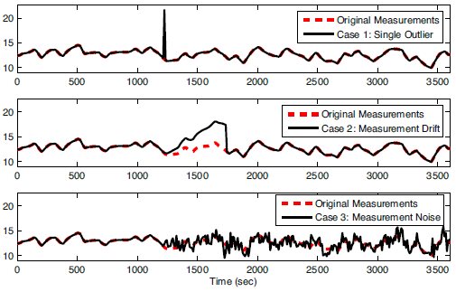
Figure 1. Example of (1) outlier, (2) drift, and (3) noise1.
Other examples of real-data issues include outliers (infrequent data points that are temporarily outside of an otherwise consistent trend in the data), noise (random variations in the data due to resolution or variations in the measurement or transmission of the data), and drift (inaccurate and gradual increase or decrease of the measurement value that does not represent the true values). Data may also be infrequent (such as measurements that occur every few hours or not at regular intervals), intermittent (such as from unreliable measurements that report good values for only certain periods of time), or time delayed (measurements that are reported after a waiting period). Synchronization of real data to process models can be challenging for all of these reasons.
Some estimators and controllers are designed with ideal measurements in simulation but then fail to perform in practice due to the issues with real measurements. It is important to use methods that perform well in a variety of situations and can either reject or minimize the effect of bad data.
Exercise
Objective: Understand the effect of bad data on dynamic optimization algorithms including estimator and control performance. Create a MATLAB or Python script to simulate and display the results. Estimated Time: 2 hours
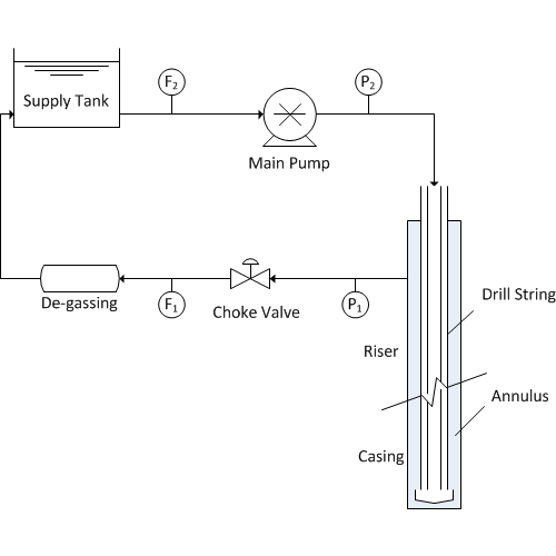
The flowrate of mud and cuttings is especially important with managed pressure drilling (MPD) in order to detect gas influx or fluid losses. There are a range of measurement instruments for flow such as a mass flow meter or Coriolis flow meter (most accurate) and a paddle wheel (least accurate). This particular system has dynamics that are described by the following equation with Cv=1, u is the valve opening, and d is a disturbance.
0.1 dF1/dt = -F1 + Cv u + d
Determine the effect of bad data (outliers, drift, and noise) on estimators such as such as moving horizon estimation. There is no need to design the estimators for this problem. The estimator scripts are below with sections that can be added to simulate the effect of bad data1. Only an outlier has been added to these code. The code should be modified to include other common phenomena such as measurement drift (gradual ramp away from the true value) and an increase in noise (random fluctuations). Comment on the effect of corrupted data on real-time estimation and why some methods are more effective at rejecting bad data.

from gekko import GEKKO
import numpy as np
import random
# intial parameters
n_iter = 150 # number of cycles
x = 37.727 # true value
# filtered bias update
alpha = 0.0951
# mhe tuning
horizon = 30
#%% Model
#Initialize model
m = GEKKO()
# Solve options
rmt = True # Remote: True or False
# For rmt=True, specify server
m.server = 'https://byu.apmonitor.com'
#time array
m.time = np.arange(50)
#Parameters
u = m.Param(value=42)
d = m.FV(value=0)
Cv = m.Param(value=1)
tau = m.Param(value=0.1)
#Variable
flow = m.CV(value=42)
#Equation
m.Equation(tau * flow.dt() == -flow + Cv * u + d)
# Options
m.options.imode = 5
m.options.ev_type = 1 #start with l1 norm
m.options.coldstart = 1
m.options.solver = 1 # APOPT solver
d.status = 1
flow.fstatus = 1
flow.wmeas = 100
flow.wmodel = 0
#flow.dcost = 0
# Initialize L1 application
m.solve(remote=rmt)
#%% Other Setup
# Create storage for results
xtrue = x * np.ones(n_iter+1)
z = x * np.ones(n_iter+1)
time = np.zeros(n_iter+1)
xb = np.empty(n_iter+1)
x1mhe = np.empty(n_iter+1)
x2mhe = np.empty(n_iter+1)
# initial estimator values
x0 = 40
xb[0] = x0
x1mhe[0] = x0
x2mhe[0] = x0
# outliers
for i in range(n_iter+1):
z[i] = x + (random.random()-0.5)*2.0
z[50] = 100
z[100] = 0
#%% L1 Application
## Cycle through measurement sequentially
for k in range(1, n_iter+1):
print( 'Cycle ' + str(k) + ' of ' + str(n_iter))
time[k] = k
# L1-norm MHE
flow.meas = z[k]
m.solve(remote=rmt)
x1mhe[k] = flow.model
print("Finished L1")
#%% L2 application
#clear L1//
m.clear_data()
# Options for L2
m.options.ev_type = 2 #start with l1 norm
m.options.coldstart = 1 #reinitialize
flow.wmodel = 10
# Initialize L2 application
m.solve(remote=rmt)
## Cycle through measurement sequentially
for k in range(1, n_iter+1):
print ('Cycle ' + str(k) + ' of ' + str(n_iter))
time[k] = k
# L2-norm MHE
flow.meas = z[k]
m.solve(remote=rmt)
x2mhe[k] = flow.model
#%% Filtered bias update
## Cycle through measurement sequentially
for k in range(1, n_iter+1):
print ('Cycle ' + str(k) + ' of ' + str(n_iter))
time[k] = k
# filtered bias update
xb[k] = alpha * z[k] + (1.0-alpha) * xb[k-1]
#%% plot results
import matplotlib.pyplot as plt
plt.figure(1)
plt.plot(time,z,'kx',lw=2)
plt.plot(time,xb,'g--',lw=3)
plt.plot(time,x2mhe,'k-',lw=3)
plt.plot(time,x1mhe,'r.-',lw=3)
plt.plot(time,xtrue,'k:',lw=2)
plt.legend(['Measurement','Filtered Bias Update','Sq Error MHE','l_1-Norm MHE','Actual Value'])
plt.xlabel('Time (sec)')
plt.ylabel('Flow Rate (T/hr)')
plt.axis([0, time[n_iter], 32, 45])
plt.show()
Solution
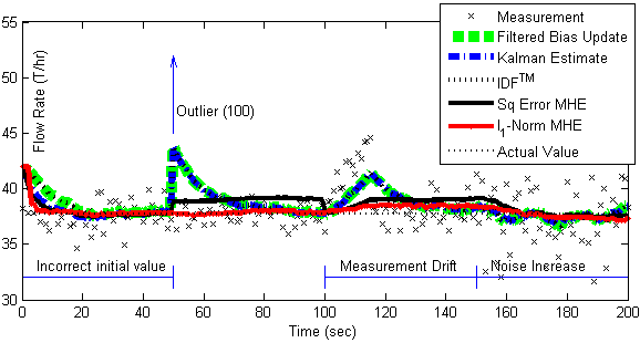
The solution shows the results of five different estimators including filtered bias update, Kalman filter, Implicit Dynamic Feedback, and Moving Horizon Estimation with a squared error or l1-norm objective.