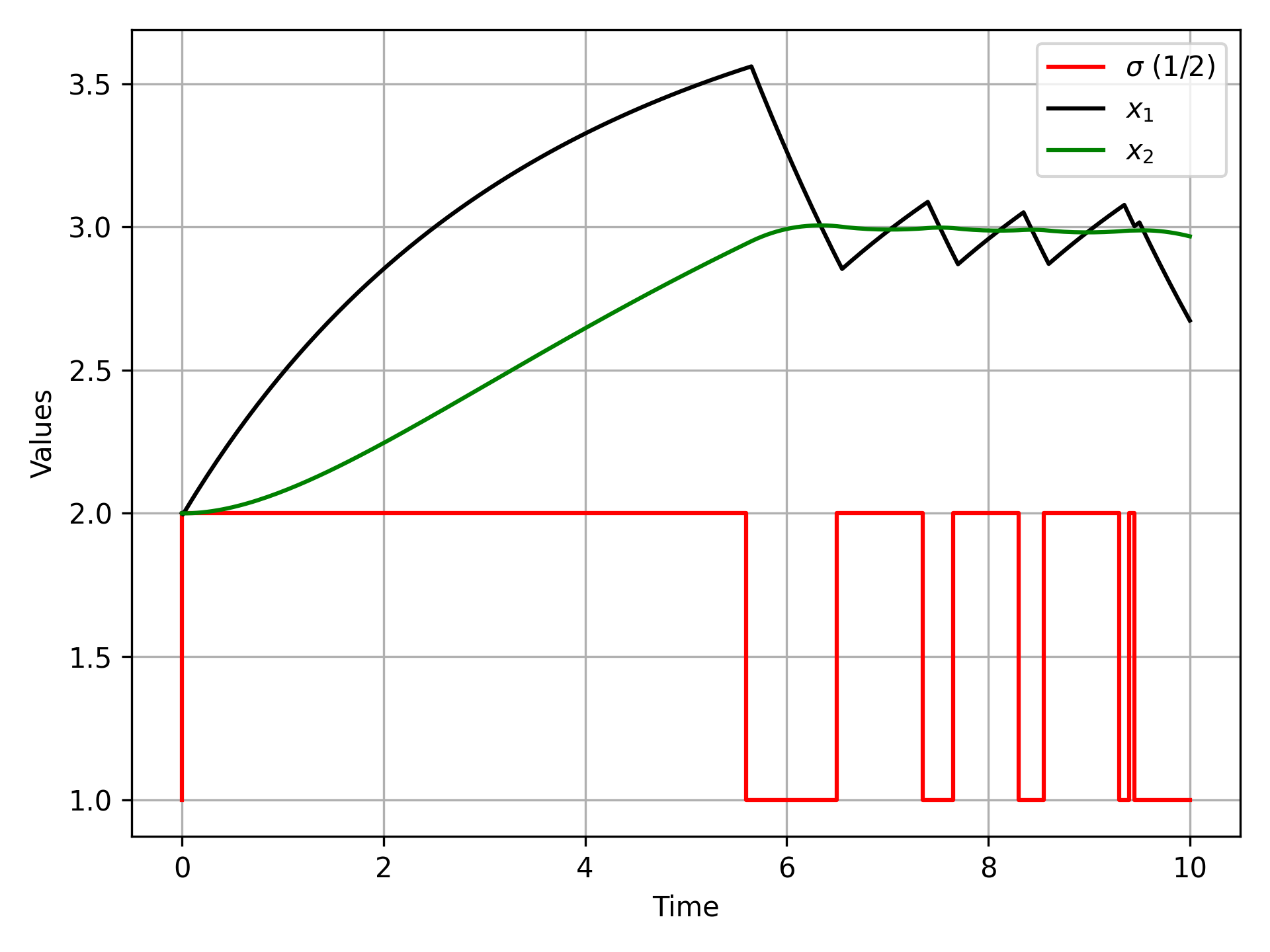
A double tank is an example of a switching system where the input to the upper tank can be one of two flows. The upper tank drains to the lower tank and the lower tank drains to a reservoir. The flow to the upper tank is the manipulated variable to meet a lower tank target level. A higher upper tank level leads to a higher flowrate into the lower tank. The dynamics of the two levels are described by two differential equations.
$$\begin{aligned}\min_\sigma \quad & \int_{0}^{T} (x_2-SP)^2 \, \text{dt} \\ \text{subject to} \quad & \frac{dx_1}{dt} = \sigma(t)-\sqrt{x_1} \\ & \frac{dx_2}{dt} = \sqrt{x_1}-\sqrt{x_2} \\ & x(0) = \begin{pmatrix} 2 \\ 2 \end{pmatrix} \\ & \sigma(t) \in \{1,2\} \quad \text{for } t \in [0,T] \end{aligned}$$
The set point is `SP=3`. The two states x are the fluid levels in the upper and a lower tank. The flow into the upper tank is either 1 or 2, the upper tank flows into the lower tank, and the lower tank flow exits the system. The objective of the optimal control problem is for the lower tank to reach the setpoint `SP` during the optimization window of 10 minutes.
import matplotlib.pyplot as plt
from gekko import GEKKO
m = GEKKO(remote=False)
# Add 0.01 as first step
# 0,0.01,0.1,0.2,0.3,...9.9,10.0)
m.time = np.insert(np.linspace(0,10,201),1,0.01)
# change solver options
m.solver_options = ['minlp_gap_tol 0.001',\
'minlp_maximum_iterations 10000',\
'minlp_max_iter_with_int_sol 100',\
'minlp_branch_method 1',\
'minlp_integer_tol 0.001',\
'minlp_integer_leaves 0',\
'minlp_maximum_iterations 200']
SP = 3
last = m.Param(np.zeros(202))
last.value[-1] = 1
sigma=m.MV(value=1,lb=1,ub=2,integer=True)
sigma.STATUS = 1
x1 = m.Var(value=2)
x2 = m.Var(value=2)
x3 = m.Var(value=0)
m.Minimize(last*x3)
m.Equations([x1.dt() == sigma - m.sqrt(x1),\
x2.dt() == m.sqrt(x1) - m.sqrt(x2),\
x3 == m.integral((x2-SP)**2)])
m.options.IMODE = 6
m.options.NODES = 3
m.options.SOLVER = 1
m.options.MV_TYPE = 0
m.solve()
plt.figure(1)
plt.step(m.time,sigma.value,'r-',label=r'$\sigma$ (1/2)')
plt.plot(m.time,x1.value,'k-',label=r'$x_1$')
plt.plot(m.time,x2.value,'g-',label=r'$x_2$')
plt.xlabel('Time'); plt.ylabel('Values')
plt.grid(); plt.legend(); plt.tight_layout()
plt.savefig('double_tank.png',dpi=300)
plt.show()
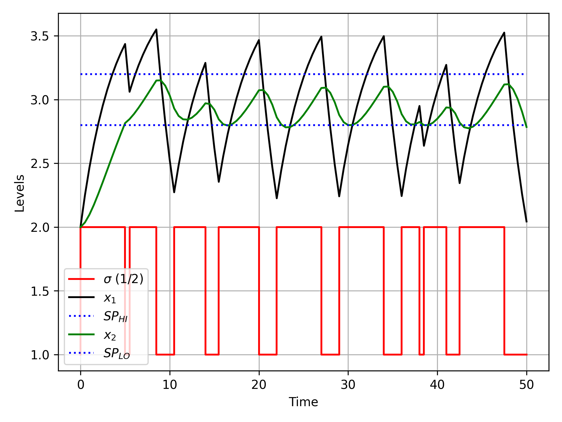
The tight set point track leads to valve chatter as small adjustments are made to keep the level at the constant value. This has several potential negative consequences including wearing out the valve with excessive travel and frequent upstream disturbances in pressure and flow. For surge tanks, a more common approach is to keep the level within a specified range such as 2.8 to 3.2. An l1-norm objective is implemented with the dead-band region to avoid valve chatter and inlet flow fluctuations. The simulation is extended to 50 minutes to observe the dead-band tracking.
import matplotlib.pyplot as plt
from gekko import GEKKO
m = GEKKO(remote=True)
# Add 0.01 as first step
m.time = np.insert(np.linspace(0,50,101),1,0.01)
# change solver options
m.solver_options = ['minlp_gap_tol 0.001',\
'minlp_maximum_iterations 10000',\
'minlp_max_iter_with_int_sol 100',\
'minlp_branch_method 1',\
'minlp_integer_tol 0.001',\
'minlp_integer_leaves 0',\
'minlp_maximum_iterations 200']
SP = 3
last = m.Param(np.zeros(102))
last.value[-1] = 1
sigma=m.MV(value=1,lb=1,ub=2,integer=True)
sigma.STATUS = 1; sigma.DCOST=1e-5
x1 = m.Var(value=2)
x2 = m.CV(value=2); x2.STATUS=1
x2.SPLO = SP-0.2; x2.SPHI = SP+0.2
m.Equations([x1.dt() == sigma - m.sqrt(x1),\
x2.dt() == m.sqrt(x1) - m.sqrt(x2)])
m.options.IMODE = 6
m.options.NODES = 2
m.options.SOLVER = 1
m.options.MV_TYPE = 0
m.solve()
plt.figure(1)
plt.step(m.time,sigma.value,'r-',label=r'$\sigma$ (1/2)')
plt.plot(m.time,x1.value,'k-',label=r'$x_1$')
plt.plot([0,m.time[-1]],[x2.SPHI,x2.SPHI],'b:',label=r'$SP_{HI}$')
plt.plot(m.time,x2.value,'g-',label=r'$x_2$')
plt.plot([0,m.time[-1]],[x2.SPLO,x2.SPLO],'b:',label=r'$SP_{LO}$')
plt.xlabel('Time'); plt.ylabel('Levels')
plt.grid(); plt.legend(); plt.tight_layout()
plt.savefig('double_tank.png',dpi=300)
plt.show()

The Gekko Optimization Suite is a machine learning and optimization package in Python for mixed-integer and differential algebraic equations.
📄 Gekko Publication and References
The GEKKO package is available in Python with pip install gekko. There are additional example problems for equation solving, optimization, regression, dynamic simulation, model predictive control, and machine learning.