Dynamic Optimization

Attach:controller_tuning.mp4

(:html:) <video width="550" controls autoplay loop>

  <source src="/do/uploads/Main/controller_tuning.mp4" type="video/mp4">
  Your browser does not support the video tag.

</video> (:htmlend:)

from IPython import get_ipython

1. detect if IPython is running

ipython = get_ipython() is not None

m = GEKKO(remote=False)

    if ipython:
        display.clear_output(wait=True)
    else:
        plt.clf()

    plt.pause(0.01)

1. Make an MP4 animation?

make_mp4 = True if make_mp4:

    import imageio  # required to make animation
    import os
    try:
        os.mkdir('./figures')
    except:
        pass

    plt.plot(tm,u.value,'k-',lw=2,label='u')
    plt.ylim([-1,11])
    plt.legend(loc=1)

    plt.plot(tm,z['x.tr_hi'],'k--',label='x traj')
    plt.plot(tm,z['x.tr_lo'],'k--')
    plt.legend(loc=1)

    plt.plot(tm,z['y.tr_hi'],'k--',label='y traj')
    plt.plot(tm,z['y.tr_lo'],'k--')
    plt.legend(loc=1)
    plt.draw()

    if make_mp4:
        filename='./figures/plot_str(i+10000).png'
        plt.savefig(filename)

1. generate mp4 from png figures

if make_mp4:

    images = []
    for i in range(40):
        filename='./figures/plot_str(i+10000).png'
        images.append(imageio.imread(filename))
    try:
        imageio.mimsave('results.mp4', images)
    except:
        print('Error: Install mp4 generator with "pip install imageio-ffmpeg"')

x.TR_INIT = 1

(:toggle hide gekko button show="Gekko Solution":) (:div id=gekko:) (:source lang=python:) import numpy as np from gekko import GEKKO import matplotlib.pyplot as plt import json from IPython import display m = GEKKO() t = np.linspace(0,15,31) m.time = t # 0.5 cycle time u = m.MV(1,name='u') x = m.CV(name='x') y = m.CV(name='y') m.Equations([5*x.dt() ==-x+1.5*u, 15*y.dt()==-y+3.0*u]) m.options.IMODE = 6 m.options.NODES = 3

1. MV tuning

u.DCOST = 0.1 u.DMAX = 1.5 u.STATUS = 1 u.FSTATUS = 0 u.UPPER = 10 u.LOWER = 0

1. CV tuning

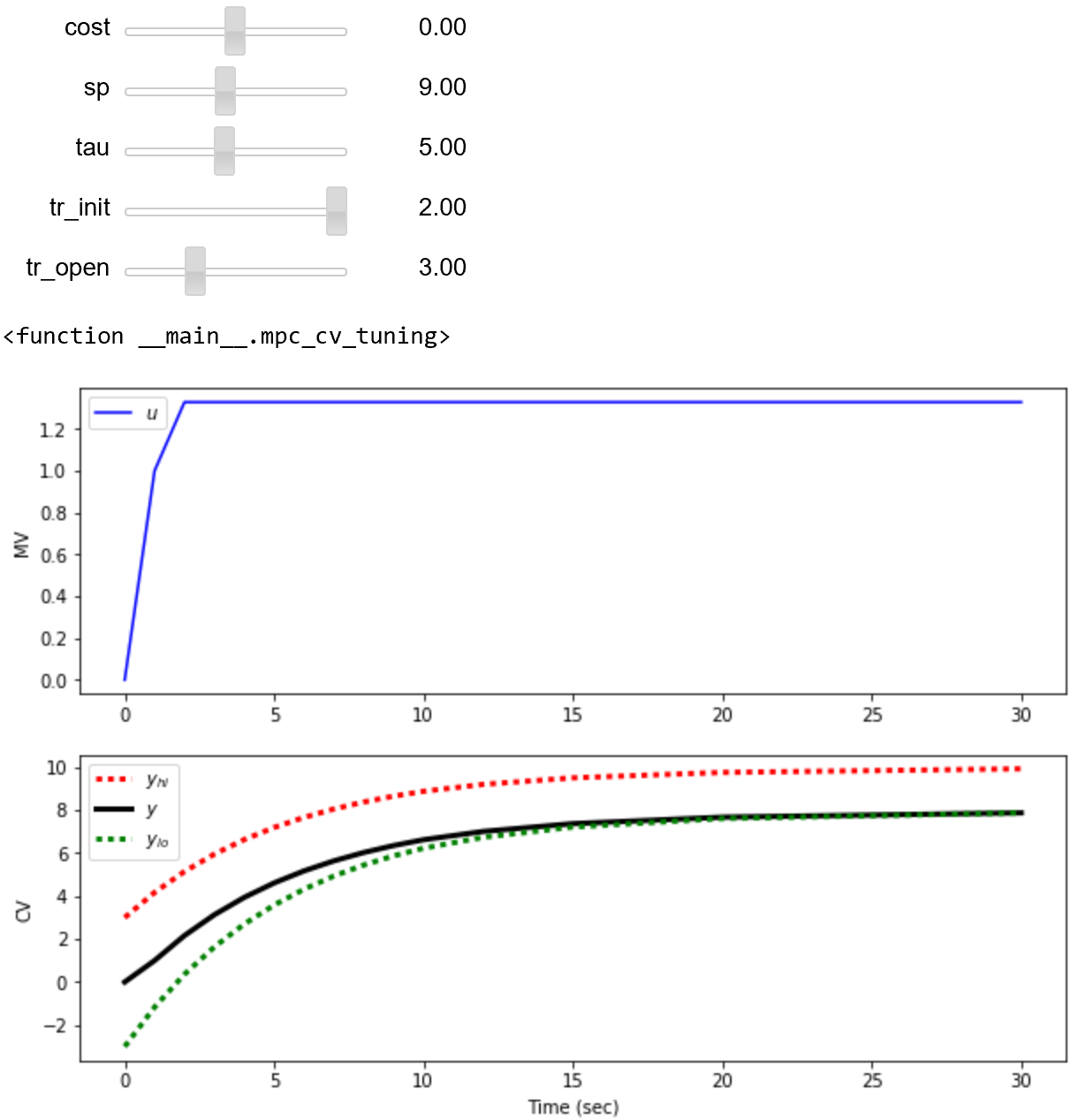
x.STATUS = 1 x.FSTATUS = 0 x.SPHI = 10 x.SPLO = 9 x.TAU = 2 x.TR_INIT = 2 x.TR_OPEN = 5 x.WSPHI = 100 x.WSPLO = 100

y.STATUS = 1 y.FSTATUS = 0 y.SPHI = 7 y.SPLO = 2 y.TAU = 0 y.TR_INIT = 0 y.TR_OPEN = 1 y.WSPHI = 200 y.WSPLO = 50

1. plot solution

plt.figure(figsize=(8,5)) plt.ion() plt.show()

for i in range(40):

    m.solve(disp=False)

    # update time
    tm = m.time+i*0.5

    # x is more important at t=10
    if tm[0]>=10:
        x.WSPLO = 500
        x.WSPHI = 500

    # get trajectory information
    with open(m.path+'//results.json') as f:
        z = json.load(f)

    display.clear_output(wait=True)
    plt.clf()
    plt.figure(1,figsize=(8,5))
    plt.subplot(3,1,1)
    plt.plot(tm,u.value,'k-',linewidth=2)
    plt.legend('u')
    plt.ylabel('MV')

    plt.subplot(3,1,2)
    plt.plot(tm,x.value,'b-',lw=2,label='x')
    plt.plot(tm,z['x.tr_hi'],'b--',label='x traj')
    plt.plot(tm,z['x.tr_lo'],'b--')
    plt.legend()

    plt.subplot(3,1,3)
    plt.plot(tm,y.value,'r-',lw=2,label='y')
    plt.plot(tm,z['y.tr_hi'],'r--',label='y traj')
    plt.plot(tm,z['y.tr_lo'],'r--')
    plt.legend()
    plt.pause(0.01)

(:sourceend:) (:divend:)

MPC Tuning Solution (APM MATLAB and APM Python

Use the following system of linear differential equations for this exercise by placing the model definition in the file myModel.apm (APMonitor) or in a Python script (Gekko).

APMonitor Model

Gekko Model

(:source lang=python:) import numpy as np from gekko import GEKKO m = GEKKO() t = np.linspace(0,15,76) m.time = t # 0.2 cycle time u = m.MV(1,name='u') x = m.CV(name='x') y = m.CV(name='y') m.Equations([5*x.dt() ==-x+1.5*u, 15*y.dt()==-y+3.0*u]) (:sourceend:)

• Application tuning

• Manipulated Variable (MV) tuning

• Controlled Variable (CV) tuning

download.png MPC Tuning IPython Widget

• SOLVER
  • 0=Try all available solvers
  • 1=APOPT (MINLP, Active Set SQP)
  • 2=BPOPT (NLP, Interior Point, SQP)
  • 3=IPOPT (NLP, Interior Point, SQP)

• COST = (+) minimize CV, (-) maximize CV

• STATUS = turn on (1) or off (0) CV

<iframe width="560" height="315" src="https://www.youtube.com/embed/JnD6kpOul1c" frameborder="0" allowfullscreen></iframe>

In this case, the parameter u is the manipulated variable and x and y are the controlled variables. It is desired to maximize x and maintain values between 9 and 10. It is desired to maintain values of y between 2 and 7. For the first 10 minutes, the priority is to maintain the range for y and following this time period, it is desired to track the range for x. Tune the controller to meet these objectives while minimizing MV movement.

• CV_TYPE = CV type with 1=l_1-norm, 2=squared error

Exercise

Objective: Design a model predictive controller with one manipulated variable and two controlled variables with competing objectives that cannot be simultaneously satisfied. Tune the controller to achieve best performance. Estimated time: 2 hours.

Use the following system of linear differential equations for this exercise by placing the model definition in the file myModel.apm.

 Parameters
  u
 Variables
  x
  y
 Equations
  5 * $x = -x + 1.5 * u
  15 * $y = -y + 3.0 * u

In this case, the parameter u is the manipulated variable and x and y are the controlled variables. It is desired to maximize x and maintain values between 9 and 10. It is desired to maintain values of y between 2 and 5. For the first 10 minutes, the priority is to maintain the range for y and following this time period, it is desired to track the range for x. Tune the controller to meet these objectives while minimizing MV movement.

Solution

(:html:) <iframe width="560" height="315" src="https://www.youtube.com/embed/yw_a9ektOqc?rel=0" frameborder="0" allowfullscreen></iframe> (:htmlend:)

• CV_TYPE = 1 for l₁-norm and 2 for squared error

• SP = set point with CV_TYPE = 2
• SPLO = lower set point with CV_TYPE = 1
• SPHI = upper set point with CV_TYPE = 1

• TR_OPEN = opening at initial point of trajectory compared to end

Common Tuning Parameters for MPC

Tuning typically involves adjustment of objective function terms or constraints that limit the rate of change (DMAX), penalize the rate of change (DCOST), or set absolute bounds (LOWER and UPPER). Measurement availability is indicated by the parameter (FSTATUS). The optimizer can also include (1=on) or exclude (0=off) a certain manipulated variable (MV) or controlled variable with STATUS. Below are common application, MV, and CV tuning constants that are adjusted to achieve desired model predictive control performance.

• Application tuning
  • IMODE = 6 or 9 for model predictive control
  • DIAGLEVEL = diagnostic level (0-10) for solution information
  • MAX_ITER = maximum iterations
  • MAX_TIME = maximum time before stopping
  • MV_TYPE = Set default MV type with 0=zero-order hold, 1=linear interpolation
• Manipulated Variable (MV) tuning
  • COST = (+) minimize MV, (-) maximize MV
  • DCOST = penalty for MV movement
  • DMAX = maximum that MV can move each cycle
  • FSTATUS = feedback status with 1=measured, 0=off
  • LOWER = lower MV bound
  • MV_TYPE = MV type with 0=zero-order hold, 1=linear interpolation
  • STATUS = turn on (1) or off (0) MV
  • UPPER = upper MV bound
• Controlled Variable (CV) tuning
  • COST = (+) minimize MV, (-) maximize MV
  • CV_TYPE = CV type with 1=l_1-norm, 2=squared error
  • FSTATUS = feedback status with 1=measured, 0=off
  • SP = setpoint with CV_TYPE = 2
  • SPLO = lower setpoint with CV_TYPE = 1
  • SPHI = upper setpoint with CV_TYPE = 1
  • STATUS = turn on (1) or off (0) MV
  • TAU = reference trajectory time-constant
  • TR_INIT = trajectory type, 0=dead-band, 1,2=trajectory
  • TR_OPEN = opening at initial point of traj compared to end

There are several ways to change the tuning values. Tuning values can either be specified before an application is initialized or while an application is running. To change a tuning value before the application is loaded, use the apm_option() function such as the following example to change the lower bound in MATLAB or Python for the MV named u.

 apm_option(server,app,'u.LOWER',0)

The upper and lower deadband targets for a CV named y are set to values around a desired set point of 10.0. In this case, an acceptable range for this CV is between 9.5 and 10.5.

 sp = 10.0
 apm_option(server,app,'y.SPHI',sp+0.5)
 apm_option(server,app,'y.SPHI',sp-0.5)

Application constants are modified by indicating that the constant belongs to the group nlc. IMODE is adjusted to either solve the MPC problem with a simultaneous (6) or sequential (9) method. In the case below, the application IMODE is changed to simultaneous mode.

 apm_option(server,app,'nlc.IMODE',6)

(:title Dynamic Control Tuning:) (:keywords tuning, Python, MATLAB, Simulink, nonlinear control, model predictive control, tutorial:) (:description Tuning of an optimizing controller for improved following of a desired trajectory or to reach an optimal state:)

Dynamic controller tuning is the process of adjusting certain objective function terms to give more desirable solutions. As an example, a dynamic control application may either exhibit too aggressive manipulated variable movement or be too sluggish during set-point changes. Tuning is the iterative process of finding acceptable values that work over a wide range of operating conditions.