{
"cells": [
{
"cell_type": "markdown",
"metadata": {},
"source": [
"## Temperature Control Lab, Python Introduction, Parts 5-7\n",
"\n",
"The TCLab (Temperature Control Lab) has an LED, two heaters, and two temperature sensors that are controlled with an Arduino. The heater power output is adjusted to maintain a desired temperature. Thermal energy from the heater is transferred by conduction, convection, and radiation to the temperature sensor. Heat is also transferred away from the device to the surroundings. This lab is a resource to learn data analysis, visualization, regression, and model analysis in Python with real data. Temperature control is an important problem in many applications such as:\n",
"\n",
"* Maintain temperature of a home during the winter\n",
"* Pre-heat an oven for baking\n",
"* Regulate the temperature in a chemical reactor\n",
"* Reduce temperature variations during semiconductor production\n",
"* Adjust the infrared heater for a newborn baby in an incubator to maintain body temperature\n",
"* Regulate natural gas to a water heater to provide consistent hot water\n",
"* Adjust flow through a heat exchanger to maintain outlet temperature\n",
"* Others?\n",
"\n",
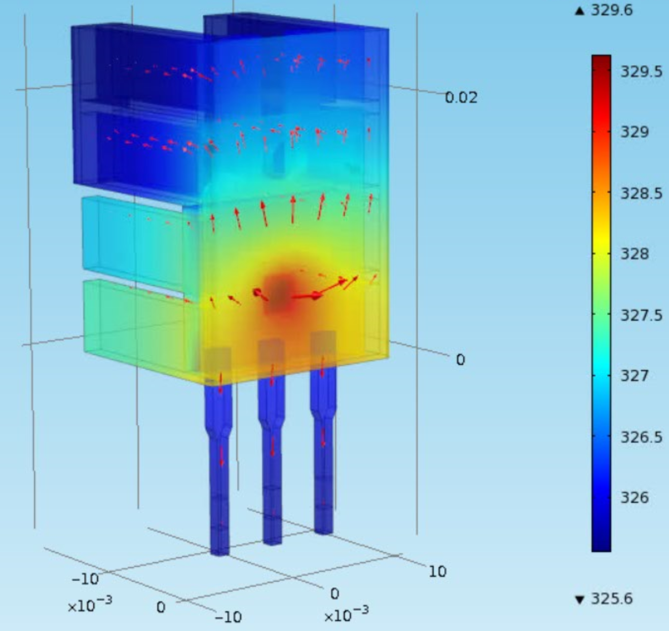
"The heaters and LED can be adjusted between 0-100% output. The dual heater effect is shown in the plot below where heat is transferred from hot to cold according to Fick's law.\n",
"\n",
"\n",
"\n",
"This Python lab is a cumulative activity that covers the following topics:\n",
"\n",
"* Part 5: Thermal Conductivity Tests\n",
"* Part 6: Energy Balance for Composite Thermal Conductivity\n",
"* Part 7: Transient Energy Balance Solution"
]
},
{
"cell_type": "markdown",
"metadata": {},
"source": [
"### Install TCLab and Load Packages\n",
"\n",
"[Retrieve tclab.py from Github](https://github.com/APMonitor/arduino/blob/master/0_Test_Device/Python/tclab/tclab.py) if pip install is not successful such as for computers where the user does not have administrative privileges to install packages. Include tclab.py in the same directory as the Jupyter notebook."
]
},
{
"cell_type": "code",
"execution_count": 1,
"metadata": {
"collapsed": true
},
"outputs": [],
"source": [
"# download tclab.py from \n",
"try:\n",
" import tclab\n",
"except:\n",
" !pip install tclab\n",
" import tclab\n",
"\n",
"# import additional packages \n",
"import time\n",
"import numpy as np\n",
"import matplotlib.pyplot as plt\n",
"%matplotlib inline\n",
"from scipy.optimize import fsolve\n",
"from scipy.integrate import odeint\n",
"from scipy.interpolate import interp1d"
]
},
{
"cell_type": "markdown",
"metadata": {},
"source": [
"### Connect Test TCLab to Computer with USB Cable\n",
"\n",
"Connect the temperature control lab with the USB cable to the computer (MacOS, Windows, or Linux). Also, attach the power supply to the __top__ barrel jack as shown below. There is an [installation guide](http://apmonitor.com/pdc/index.php/Main/ArduinoSetup) if the connection is unsuccessful.\n",
"\n",
"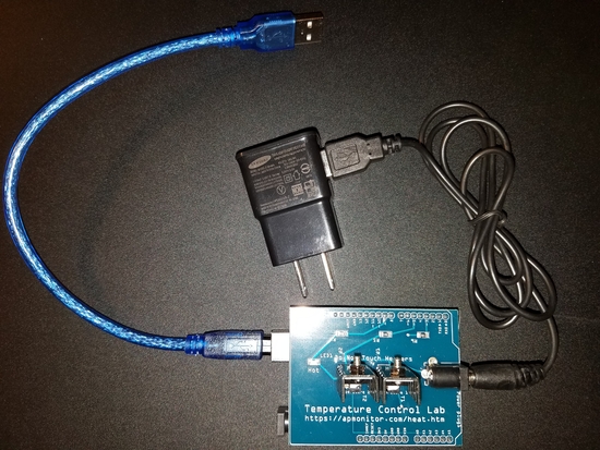 "
]
},
{
"cell_type": "code",
"execution_count": 2,
"metadata": {
"collapsed": false
},
"outputs": [
{
"name": "stdout",
"output_type": "stream",
"text": [
"TCLab version 0.4.6\n",
"Arduino Leonardo connected on port COM13 at 115200 baud.\n",
"TCLab Firmware Version 1.01.\n",
"T1: 24.77\n",
"T2: 23.8\n",
"TCLab disconnected successfully.\n"
]
}
],
"source": [
"with tclab.TCLab() as lab:\n",
" for i in range(5):\n",
" lab.LED(100) # Turn on LED (0-100%)\n",
" time.sleep(0.5) # Pause for 0.5 second\n",
" lab.LED(0) # Turn off LED\n",
" time.sleep(0.5) # Pause for 0.5 second\n",
" print('T1: ' + str(lab.T1))\n",
" print('T2: ' + str(lab.T2)) "
]
},
{
"cell_type": "markdown",
"metadata": {},
"source": [
"## Parts 1-4\n",
"\n",
"Parts 1-4 should be completed before this lab.\n",
"\n",
"Part 1 covers Python loops, files, and plotting. Part 2 covers linear, nonlinear, and nonlinear regression. A Jupyter notebook for Parts 1 and 2 is available at the following link:\n",
"\n",
"[Jupyter Notebook for TCLab Parts 1 and 2](https://nbviewer.jupyter.org/url/apmonitor.com/che263/uploads/Main/TCLab_A.ipynb)\n",
"\n",
"Part 3 covers interpolation and part 4 involves linear, nonlinear, and differential equation solving. A Jupyter notebook for Parts 3 and 4 is available at the following link:\n",
"\n",
"[Jupyter Notebook for TCLab Parts 3 and 4](https://nbviewer.jupyter.org/url/apmonitor.com/che263/uploads/Main/TCLab_B.ipynb)"
]
},
{
"cell_type": "markdown",
"metadata": {},
"source": [
"## Part 5: Thermal Conductivity\n",
"\n",
""
]
},
{
"cell_type": "markdown",
"metadata": {},
"source": [
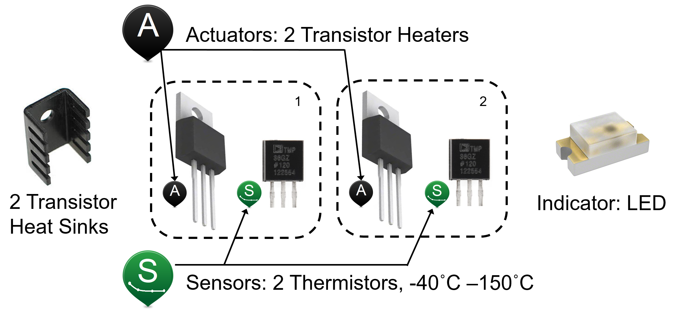
"### A: Material Test Data\n",
"\n",
"Insert metal coins, plastic, and cardboard in between the two heaters so that there is a conduction path for heat between the two sensors. The temperature difference and temperature levels are affected by the ability of the material to conduct heat from heater 1 and temperature sensor $(T_1)$ to the other temperature sensor $(T_2)$.\n",
"\n",
"Turn on heater 1 to 100% and record $T_1$, $T_2$, and the temperature difference $\\Delta T = T_1-T_2$ every 10 seconds for 8 minutes for each material (6 x 8 + 1 = 49 data points). The objective is to observe the temperatures at steady state conditions and longer or shorter tests may be required to reach steady state. For each material test, record the values at the end after the system has reached a steady state equilibrium.\n",
"\n",
"When changing out the materials between the heaters, wait until the heaters have cooled off and avoid touching a hot surface. There are thermochromic paint dots on the heaters that turn pink when the heaters are above 37$^oC$ (99$^oF$). Do not touch the heaters or the material between the heaters directly after the test. Blowing on the heaters helps to cool them quickly."
]
},
{
"cell_type": "markdown",
"metadata": {},
"source": [
"### B: Analyze Data\n",
"\n",
"Locate the thermal conductivity of the materials inserted between the heaters. Below are some common materials with thermal conductivities.\n",
"\n",
"| __Material__ | __Thermal Conductivity $\\left(\\frac{W}{m\\;K}\\right)$__ |\n",
"|------|------|\n",
"| Aluminum | 237 |\n",
"| Cardboard / Paper | 0.05 |\n",
"| Copper (US Penny <1981) | 401 |\n",
"| Gold | 318 |\n",
"| Plastic (LDPE) | 0.36 |\n",
"| Silver | 429 |\n",
"| Stainless Steel | 18 |\n",
"| Steel (<0.5% Carbon) | 54 |\n",
"| Zinc (US Penny >1983) | 116 |\n",
"\n",
"Create a semi-log x plot of the thermal conductivity versus $T_1$, $T_2$, and $\\Delta T$ using an average of the last 6 data points for each of the plastic, metal, and cardboard tests. Use __plt.semilogx__ to create the plot with thermal conductivity as the first argument and the temperatures as the second argument."
]
},
{
"cell_type": "markdown",
"metadata": {},
"source": [
"### C: Regression\n",
"\n",
"Create a linear regression for $\\log_{10}$(thermal conductivity) versus $T_1$, $T_2$, and $\\Delta T$. Predict the steady state $T_1$, $T_2$, and $\\Delta T$ for stainless steel using the linear model."
]
},
{
"cell_type": "markdown",
"metadata": {},
"source": [
"### D: Explain Linear Model Slope\n",
"\n",
"Display the slope of each of the linear models for $\\log_{10}$(thermal conductivity) versus $T_1$, $T_2$, and $\\Delta T$. Based on heat transfer principles, explain the sign (positive or negative) of the slope. In other words, why does the temperature either increase or decrease with increasing thermal conductivity?"
]
},
{
"cell_type": "markdown",
"metadata": {},
"source": [
"## Part 6: Composite Thermal Conductivity $(k_c)$"
]
},
{
"cell_type": "markdown",
"metadata": {},
"source": [
"An energy balance includes energy accumulation $m \\, c_p \\, \\frac{dT}{dt}$, energy in, and energy out. The energy balance includes conduction from $T_1$ (+energy), convection to the ambient air (-energy), and radiative heat transfer (-energy). Use the following equations for an energy balance on $T_2$. \n",
"\n",
"Conduction (Fourier's Law): $q_{cond} = -k \\frac{dT}{dx} \\approx -k_c \\frac{T_2-T_1}{\\Delta x}$\n",
"\n",
"Convective Heat Transfer: $q_{conv} = h \\, A \\, \\left(T_\\infty-T_2\\right)$\n",
"\n",
"Radiative Heat Transfer: $q_{rad} = \\sigma \\, \\epsilon \\, A \\, \\left((T_\\infty+273.15)^4-(T_2+273.15)^4\\right)$\n",
"\n",
"Energy Balance: $m \\, c_p \\, \\frac{dT_2}{dt} = q_{cond} + q_{conv} + q_{rad}$\n",
"\n",
"
"
]
},
{
"cell_type": "code",
"execution_count": 2,
"metadata": {
"collapsed": false
},
"outputs": [
{
"name": "stdout",
"output_type": "stream",
"text": [
"TCLab version 0.4.6\n",
"Arduino Leonardo connected on port COM13 at 115200 baud.\n",
"TCLab Firmware Version 1.01.\n",
"T1: 24.77\n",
"T2: 23.8\n",
"TCLab disconnected successfully.\n"
]
}
],
"source": [
"with tclab.TCLab() as lab:\n",
" for i in range(5):\n",
" lab.LED(100) # Turn on LED (0-100%)\n",
" time.sleep(0.5) # Pause for 0.5 second\n",
" lab.LED(0) # Turn off LED\n",
" time.sleep(0.5) # Pause for 0.5 second\n",
" print('T1: ' + str(lab.T1))\n",
" print('T2: ' + str(lab.T2)) "
]
},
{
"cell_type": "markdown",
"metadata": {},
"source": [
"## Parts 1-4\n",
"\n",
"Parts 1-4 should be completed before this lab.\n",
"\n",
"Part 1 covers Python loops, files, and plotting. Part 2 covers linear, nonlinear, and nonlinear regression. A Jupyter notebook for Parts 1 and 2 is available at the following link:\n",
"\n",
"[Jupyter Notebook for TCLab Parts 1 and 2](https://nbviewer.jupyter.org/url/apmonitor.com/che263/uploads/Main/TCLab_A.ipynb)\n",
"\n",
"Part 3 covers interpolation and part 4 involves linear, nonlinear, and differential equation solving. A Jupyter notebook for Parts 3 and 4 is available at the following link:\n",
"\n",
"[Jupyter Notebook for TCLab Parts 3 and 4](https://nbviewer.jupyter.org/url/apmonitor.com/che263/uploads/Main/TCLab_B.ipynb)"
]
},
{
"cell_type": "markdown",
"metadata": {},
"source": [
"## Part 5: Thermal Conductivity\n",
"\n",
""
]
},
{
"cell_type": "markdown",
"metadata": {},
"source": [
"### A: Material Test Data\n",
"\n",
"Insert metal coins, plastic, and cardboard in between the two heaters so that there is a conduction path for heat between the two sensors. The temperature difference and temperature levels are affected by the ability of the material to conduct heat from heater 1 and temperature sensor $(T_1)$ to the other temperature sensor $(T_2)$.\n",
"\n",
"Turn on heater 1 to 100% and record $T_1$, $T_2$, and the temperature difference $\\Delta T = T_1-T_2$ every 10 seconds for 8 minutes for each material (6 x 8 + 1 = 49 data points). The objective is to observe the temperatures at steady state conditions and longer or shorter tests may be required to reach steady state. For each material test, record the values at the end after the system has reached a steady state equilibrium.\n",
"\n",
"When changing out the materials between the heaters, wait until the heaters have cooled off and avoid touching a hot surface. There are thermochromic paint dots on the heaters that turn pink when the heaters are above 37$^oC$ (99$^oF$). Do not touch the heaters or the material between the heaters directly after the test. Blowing on the heaters helps to cool them quickly."
]
},
{
"cell_type": "markdown",
"metadata": {},
"source": [
"### B: Analyze Data\n",
"\n",
"Locate the thermal conductivity of the materials inserted between the heaters. Below are some common materials with thermal conductivities.\n",
"\n",
"| __Material__ | __Thermal Conductivity $\\left(\\frac{W}{m\\;K}\\right)$__ |\n",
"|------|------|\n",
"| Aluminum | 237 |\n",
"| Cardboard / Paper | 0.05 |\n",
"| Copper (US Penny <1981) | 401 |\n",
"| Gold | 318 |\n",
"| Plastic (LDPE) | 0.36 |\n",
"| Silver | 429 |\n",
"| Stainless Steel | 18 |\n",
"| Steel (<0.5% Carbon) | 54 |\n",
"| Zinc (US Penny >1983) | 116 |\n",
"\n",
"Create a semi-log x plot of the thermal conductivity versus $T_1$, $T_2$, and $\\Delta T$ using an average of the last 6 data points for each of the plastic, metal, and cardboard tests. Use __plt.semilogx__ to create the plot with thermal conductivity as the first argument and the temperatures as the second argument."
]
},
{
"cell_type": "markdown",
"metadata": {},
"source": [
"### C: Regression\n",
"\n",
"Create a linear regression for $\\log_{10}$(thermal conductivity) versus $T_1$, $T_2$, and $\\Delta T$. Predict the steady state $T_1$, $T_2$, and $\\Delta T$ for stainless steel using the linear model."
]
},
{
"cell_type": "markdown",
"metadata": {},
"source": [
"### D: Explain Linear Model Slope\n",
"\n",
"Display the slope of each of the linear models for $\\log_{10}$(thermal conductivity) versus $T_1$, $T_2$, and $\\Delta T$. Based on heat transfer principles, explain the sign (positive or negative) of the slope. In other words, why does the temperature either increase or decrease with increasing thermal conductivity?"
]
},
{
"cell_type": "markdown",
"metadata": {},
"source": [
"## Part 6: Composite Thermal Conductivity $(k_c)$"
]
},
{
"cell_type": "markdown",
"metadata": {},
"source": [
"An energy balance includes energy accumulation $m \\, c_p \\, \\frac{dT}{dt}$, energy in, and energy out. The energy balance includes conduction from $T_1$ (+energy), convection to the ambient air (-energy), and radiative heat transfer (-energy). Use the following equations for an energy balance on $T_2$. \n",
"\n",
"Conduction (Fourier's Law): $q_{cond} = -k \\frac{dT}{dx} \\approx -k_c \\frac{T_2-T_1}{\\Delta x}$\n",
"\n",
"Convective Heat Transfer: $q_{conv} = h \\, A \\, \\left(T_\\infty-T_2\\right)$\n",
"\n",
"Radiative Heat Transfer: $q_{rad} = \\sigma \\, \\epsilon \\, A \\, \\left((T_\\infty+273.15)^4-(T_2+273.15)^4\\right)$\n",
"\n",
"Energy Balance: $m \\, c_p \\, \\frac{dT_2}{dt} = q_{cond} + q_{conv} + q_{rad}$\n",
"\n",
" \n",
"\n",
"| __Parameter__ | __Value__ |\n",
"|------|------|\n",
"| Ambient Temperature $(T_\\infty)$ | 23.0 $^oC$ |\n",
"| Distance Between Sensors $(\\Delta x)$ | 0.015 $m$ |\n",
"| Emissivity $(\\epsilon)$ | 0.9 |\n",
"| Heat Capacity $(c_p)$ | 500 $\\frac{J}{kg \\, K}$ |\n",
"| Convective Heat Transfer Coefficient $(h)$ | 4.05 $\\frac{W}{m^2 \\, K}$ |\n",
"| Mass $(m)$ | 0.004 $kg$ |\n",
"| Stefan Boltzmann Constant $(\\sigma)$ | 5.67x10$^{-8}$ $\\frac{W}{m^2 \\, K^4}$ |\n",
"| Surface Area $(A)$ | 1.0x10$^{-3}$ $m^2$ |\n",
"| Thermal Conductivity $(k)$ | Varies with Material |\n",
"\n",
"
\n",
"\n",
"| __Parameter__ | __Value__ |\n",
"|------|------|\n",
"| Ambient Temperature $(T_\\infty)$ | 23.0 $^oC$ |\n",
"| Distance Between Sensors $(\\Delta x)$ | 0.015 $m$ |\n",
"| Emissivity $(\\epsilon)$ | 0.9 |\n",
"| Heat Capacity $(c_p)$ | 500 $\\frac{J}{kg \\, K}$ |\n",
"| Convective Heat Transfer Coefficient $(h)$ | 4.05 $\\frac{W}{m^2 \\, K}$ |\n",
"| Mass $(m)$ | 0.004 $kg$ |\n",
"| Stefan Boltzmann Constant $(\\sigma)$ | 5.67x10$^{-8}$ $\\frac{W}{m^2 \\, K^4}$ |\n",
"| Surface Area $(A)$ | 1.0x10$^{-3}$ $m^2$ |\n",
"| Thermal Conductivity $(k)$ | Varies with Material |\n",
"\n",
" \n",
"\n",
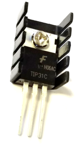
"Heat is conducted from one sensor to the other through multiple layers of varying thermal conductivity as found in the heat sink, TIP31C transistor heater, TMP36 temperature sensor, as well as the gap between the two heat sinks (air, cardboard, plastic, metal, or something else). In addition, there are 3D aspects to the heaters that should be considered with a more rigorous analysis. A more detailed model would be required to accurately predict the resistance to conductive heat transfer without validating data.\n",
"\n",
"
\n",
"\n",
"Heat is conducted from one sensor to the other through multiple layers of varying thermal conductivity as found in the heat sink, TIP31C transistor heater, TMP36 temperature sensor, as well as the gap between the two heat sinks (air, cardboard, plastic, metal, or something else). In addition, there are 3D aspects to the heaters that should be considered with a more rigorous analysis. A more detailed model would be required to accurately predict the resistance to conductive heat transfer without validating data.\n",
"\n",
" \n",
"\n",
"Instead of the more detailed analysis, determine a composite heat transfer coefficient $k_c$ for each material test with the steady state data points. For steady state, assume that $\\frac{dT_2}{dt}=0$. Solve the energy balance equation $0 = q_{conv}+q_{cond}+q_{rad}$ for $k_c$. Evaluate $k_c$ either through algebraic rearrangement or with an equation solver such as __fsolve__.\n",
"\n",
"Create a semi-log x plot of the ___composite___ thermal conductivity $(k_c)$ versus $T_1$, $T_2$, and $\\Delta T$ using an average of the last 6 data points for each of the plastic, metal, and cardboard tests. Use __plt.semilogx__ to create the plot with thermal conductivity as the first argument and the temperatures as the second argument."
]
},
{
"cell_type": "markdown",
"metadata": {},
"source": [
"## Part 7: Transient Energy Balance\n",
"\n",
"Use the composite thermal conductivity $k_c$ from the prior problem to solve the transient energy balance as an ordinary differential equation (ODE).\n",
"\n",
"Conduction (Fourier's Law): $q_{cond} = -k \\frac{dT}{dx} \\approx -k_c \\frac{T_2-T_1}{\\Delta x}$\n",
"\n",
"Convective Heat Transfer: $q_{conv} = h \\, A \\, \\left(T_\\infty-T_2\\right)$\n",
"\n",
"Radiative Heat Transfer: $q_{rad} = \\sigma \\, \\epsilon \\, A \\, \\left((T_\\infty+273.15)^4-(T_2+273.15)^4\\right)$\n",
"\n",
"Energy Balance: $m \\, c_p \\, \\frac{dT_2}{dt} = q_{cond} + q_{conv} + q_{rad}$\n",
"\n",
"The initial condition is the initial temperature of $T_2$. Show the ODE solution for $T_2$ with data for each of the 3 cases (cardboard, plastic, and metal). Plot the measured temperatures and predicted temperatures for each case in a separate subplot. Add appropriate labels to the plot."
]
}
],
"metadata": {
"kernelspec": {
"display_name": "Python 3",
"language": "python",
"name": "python3"
},
"language_info": {
"codemirror_mode": {
"name": "ipython",
"version": 3
},
"file_extension": ".py",
"mimetype": "text/x-python",
"name": "python",
"nbconvert_exporter": "python",
"pygments_lexer": "ipython3",
"version": "3.6.0"
},
"varInspector": {
"cols": {
"lenName": 16,
"lenType": 16,
"lenVar": 40
},
"kernels_config": {
"python": {
"delete_cmd_postfix": "",
"delete_cmd_prefix": "del ",
"library": "var_list.py",
"varRefreshCmd": "print(var_dic_list())"
},
"r": {
"delete_cmd_postfix": ") ",
"delete_cmd_prefix": "rm(",
"library": "var_list.r",
"varRefreshCmd": "cat(var_dic_list()) "
}
},
"types_to_exclude": [
"module",
"function",
"builtin_function_or_method",
"instance",
"_Feature"
],
"window_display": false
}
},
"nbformat": 4,
"nbformat_minor": 1
}
\n",
"\n",
"Instead of the more detailed analysis, determine a composite heat transfer coefficient $k_c$ for each material test with the steady state data points. For steady state, assume that $\\frac{dT_2}{dt}=0$. Solve the energy balance equation $0 = q_{conv}+q_{cond}+q_{rad}$ for $k_c$. Evaluate $k_c$ either through algebraic rearrangement or with an equation solver such as __fsolve__.\n",
"\n",
"Create a semi-log x plot of the ___composite___ thermal conductivity $(k_c)$ versus $T_1$, $T_2$, and $\\Delta T$ using an average of the last 6 data points for each of the plastic, metal, and cardboard tests. Use __plt.semilogx__ to create the plot with thermal conductivity as the first argument and the temperatures as the second argument."
]
},
{
"cell_type": "markdown",
"metadata": {},
"source": [
"## Part 7: Transient Energy Balance\n",
"\n",
"Use the composite thermal conductivity $k_c$ from the prior problem to solve the transient energy balance as an ordinary differential equation (ODE).\n",
"\n",
"Conduction (Fourier's Law): $q_{cond} = -k \\frac{dT}{dx} \\approx -k_c \\frac{T_2-T_1}{\\Delta x}$\n",
"\n",
"Convective Heat Transfer: $q_{conv} = h \\, A \\, \\left(T_\\infty-T_2\\right)$\n",
"\n",
"Radiative Heat Transfer: $q_{rad} = \\sigma \\, \\epsilon \\, A \\, \\left((T_\\infty+273.15)^4-(T_2+273.15)^4\\right)$\n",
"\n",
"Energy Balance: $m \\, c_p \\, \\frac{dT_2}{dt} = q_{cond} + q_{conv} + q_{rad}$\n",
"\n",
"The initial condition is the initial temperature of $T_2$. Show the ODE solution for $T_2$ with data for each of the 3 cases (cardboard, plastic, and metal). Plot the measured temperatures and predicted temperatures for each case in a separate subplot. Add appropriate labels to the plot."
]
}
],
"metadata": {
"kernelspec": {
"display_name": "Python 3",
"language": "python",
"name": "python3"
},
"language_info": {
"codemirror_mode": {
"name": "ipython",
"version": 3
},
"file_extension": ".py",
"mimetype": "text/x-python",
"name": "python",
"nbconvert_exporter": "python",
"pygments_lexer": "ipython3",
"version": "3.6.0"
},
"varInspector": {
"cols": {
"lenName": 16,
"lenType": 16,
"lenVar": 40
},
"kernels_config": {
"python": {
"delete_cmd_postfix": "",
"delete_cmd_prefix": "del ",
"library": "var_list.py",
"varRefreshCmd": "print(var_dic_list())"
},
"r": {
"delete_cmd_postfix": ") ",
"delete_cmd_prefix": "rm(",
"library": "var_list.r",
"varRefreshCmd": "cat(var_dic_list()) "
}
},
"types_to_exclude": [
"module",
"function",
"builtin_function_or_method",
"instance",
"_Feature"
],
"window_display": false
}
},
"nbformat": 4,
"nbformat_minor": 1
}