Programming Assignments
Main.CourseHomework History
Hide minor edits - Show changes to markup
Complete the following assignments with Microsoft Excel or Google Sheet (1-6) and Python for (1-17). The first 6 assignments are the same problems but completed with both a Spreadsheet program (Excel or Google Sheets) and Python. Solutions are shown for each problem but should only be used as a learning resource, not to merely complete the assignment.
Complete the following assignments with Microsoft Excel or Google Sheet (1-6) and Python for (1-17). The first 6 assignments are the same problems but completed with both a Spreadsheet program (Excel or Google Sheets) and Python. Solutions are shown for each problem but should only be used as a learning resource, not to merely complete the assignment. Join Online for homework help sessions.
Python Solutions
Python Solutions 1-2+
Python Solution 3
(:table border=0 frame=hsides width=95%:)
(:cell width=10%:)
(:table border=0 frame=hsides width=100%:)
(:cell width=5%:)
(:cell width=30%:)
(:cell width=35%:)
Excel Assignments
Complete the following assignments with Microsoft Excel, Google Sheets, or another similar spreadsheet program. Microsoft Excel solutions are shown for each problem but should only be used as a learning resource, not to merely complete the assignment. Python solutions are shown as examples of programming but are not required.
Excel and Python Assignments
Complete the following assignments with Microsoft Excel or Google Sheet (1-6) and Python for (1-17). The first 6 assignments are the same problems but completed with both a Spreadsheet program (Excel or Google Sheets) and Python. Solutions are shown for each problem but should only be used as a learning resource, not to merely complete the assignment.
Google Colab 1
Google Colab 2
Google Colab 3
Google Colab 4
Google Colab 5
Google Colab 6
Python Solutions
Python Solutions
Python Solution 2
Python Solutions
Python Solutions
Python Solutions
Python Solutions
Python Solutions 1-2
Python Solution 3
Python Solutions
(:cell width=25%:)
(:cell width=10%:) (:cell width=30%:)
(:cell width=35%:) Knowledge Building
Knowledge Building (:cell width=30%:)
1 (:cell:)
2 (:cell:)
3 (:cell:)
4 (:cell:)
5 (:cell:)
6 (:cell:)
7 (:cell:)
8 (:cell:)
9 (:cell:)
10 (:cell:)
11 (:cell:)
12 (:cell:)
13 (:cell:)
14 (:cell:)
15 (:cell:)
16 (:cell:)
17 (:cell:)
Solution 1
Solution 2
Solution 3
Soluiton 4
Python Solution 1
Python Solution 2
Python Solution 3
Python Solution 4
Google Colab 9(:cell:)
Google Colab 9 (:cell:)
Python Solutions
Python Solutions
Python Solutions
Python Solutions
Excel Solution 1
Excel Solution 2
Python Solutions
Google Colab 7
Solution 1
Solution 2
Solution 3
Soluiton 4
Google Colab 8
Python Solutions
Google Colab 9(:cell:) Generate Plots
(:cell:)
Python Solution 1
Python Solution 2
Python Solution 3
Python Solution 4
Google Colab 10
Temperature Control Lab
Python Solution 1
Python Solution 2
Google Colab 11
Python Solutions 1-5
Python Solution 6
Google Colab 12
Python Solutions 1-2
Python Solution 3
Google Colab 13
Classes (collections of values and functions)
Python Solutions 1
Python Solutions 2
Google Colab 14
Python Solutions 1-2
Python Solution 3
Python Solution 4
Google Colab 15
Python Solution 1
Python Solutions 2-4
Google Colab 16
Python Solution
Google Colab 17
Symbolic Derivatives
Integrals
(:cellnr:) (:cell:) (:cell:)
(:cellnr:) (:cell:) (:cell:)
(:cellnr:) (:cell:) (:cell:)
(:cellnr:) (:cell:) (:cell:)
Python Solution
- Assignment #1
- Conditionals
- Functions
- Excel Solution 2, Solution 3
- (:toggle hide hw1_2 button show="Solution 2 (Python)":)
(:div id=hw1_2:) (:source lang=python:)
- constants
L = 2 # m Tplate = 343 # K v = 1.45 # m/s Twater = 294 # K mu = 9.79e-4 # Pa*s rho = 998 # kg/m^3 k = 0.601 # W/m-K cp = 4.18e3 # J/kg-K
- derived quantities
Re = rho*L*v/mu Pr = mu*cp/k Nu = 0.332 * Pr**(1.0/3.0) * Re**(1.0/2.0) h = Nu * k / L q = h * (Tplate-Twater)
print('Rate of Heat Transfer') print(str(q)+' W/m^2') (:sourceend:) (:divend:)
- (:toggle hide hw1_3 button show="Solution 3 (Python)":)
(:div id=hw1_3:)
(:source lang=python:) import numpy as np import matplotlib.pyplot as plt
- calculate initial moles of N2
T = 298.15 # K P = 1.25 # atm V = 4000 # L Rg = 0.0821 # L*atm/mol/K n_N2 = P*V/(Rg*T) # moles of N2 n_N2 = n_N2 * 0.25 # moles with 25% remaining
- calculate N2 pressure at different V and T
n = 20 # grid points V = np.linspace(500,1000,n) T = np.linspace(100,600,n)
- create meshgrid
Vm,Tm = np.meshgrid(V,T)
- calculate pressure
Pm = n_N2 * Rg * Tm / Vm
- plot results
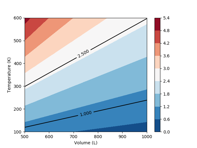
plt.figure() plt.contourf(Vm,Tm,Pm,cmap='RdBu_r') plt.colorbar() CS2 = plt.contour(Vm,Tm,Pm,[1.0,2.5],colors='k') plt.clabel(CS2, inline=1, fontsize=10) plt.xlabel('Volume (L)') plt.ylabel('Temperature (K)') plt.show() (:sourceend:) (:divend:)
- Assignment #2 - Problem 2 Data File
- Generate Plots
- Data Analysis
- Excel Solution 1, Solution 2, Solution 3
- (:toggle hide hw2_1 button show="Solution 1 (Python)":)
(:div id=hw2_1:) (:source lang=python:) import pandas as pd import matplotlib.pyplot as plt import numpy as np
- import April 2018 data or get new data from finance.yahoo.com
appl = pd.read_csv('https://apmonitor.com/che263/uploads/Main/AAPL.csv') goog = pd.read_csv('https://apmonitor.com/che263/uploads/Main/GOOG.csv')
- xom = pd.read_csv('https://apmonitor.com/che263/uploads/Main/XOM.csv')
- create dictionary of stocks
s = dict([('Apple',appl),('Google',goog)]) #,('ExxonMobil',xom)])
- print column headers and starting rows (5 is default)
print('Apple Data') print(s['Apple'].head())
- print column headers and ending close price (4 rows)
print('Google Data') print(s['Google']['Close'].tail(4))
- basic data statistics
for i in s:
    print('Stock: ' + i)
    print(' max   : ' + str(max(s[i]['Close'])))
    print(' min   : ' + str(min(s[i]['Close'])))
    print(' stdev : ' + str(np.std(s[i]['Close'])))
    print(' avg   : ' + str(np.mean(s[i]['Close'])))
    print(' median: ' + str(np.median(s[i]['Close'])))
- plot data
plt.figure() sty = dict([('Apple','r--'),('Google','b:'),('ExxonMobil','k-')]) ni = 0 for i in s:
    mc = max(s[i]['Close'])
    plt.plot(s[i]['Date'],s[i]['Close']/mc,sty[i],linewidth=3,label=i)
    plt.plot(s[i]['Date'],s[i]['High']/mc,sty[i],linewidth=1)
    plt.plot(s[i]['Date'],s[i]['Low']/mc,sty[i],linewidth=1)
plt.xticks(rotation=90) plt.legend(loc='best') plt.show() (:sourceend:) (:divend:)
- (:toggle hide hw2_2 button show="Solution 2 (Python)":)
(:div id=hw2_2:) (:source lang=python:) import pandas as pd import matplotlib.pyplot as plt
- import data
- Time (sec), Heater 1, Heater 2, Temperature 1, Temperature 2
x = pd.read_csv('https://apmonitor.com/che263/uploads/Main/tclab.txt')
- print column headers and starting 10 rows (5 is default)
print('Data') print(x.head(10))
- plot data
plt.figure() plt.subplot(2,1,1) plt.title('Temperature Control Lab') plt.plot(x['Time (sec)'],x['Temperature 1'],'r--') plt.plot(x['Time (sec)'],x['Temperature 2'],'b-') plt.ylabel('Temp (degC)') plt.legend(loc='best')
plt.subplot(2,1,2) plt.plot(x['Time (sec)'],x['Heater 1'],'r--') plt.plot(x['Time (sec)'],x['Heater 2'],'b-') plt.ylabel('Heater (%)') plt.xlabel('Time (sec)') plt.legend(loc='best') plt.show() (:sourceend:) (:divend:)
- (:toggle hide hw2_3 button show="Solution 3 (Python)":)
(:div id=hw2_3:) (:source lang=python:) import math as m
- part a
help(m.cos) y = m.cos(0.5) print('cos(0.5): ' + str(y))
- part b
y = m.sin(30.0*(m.pi/180.0)) print('sin(30 deg): ' + str(y))
- part c
y = m.tan(m.pi/2.0) print('tan(pi/x): ' + str(y))
- part d
x = 5.0 y = max(2.0*m.sqrt(x),(x**2)/2.0, (x**3)/3.0,(x**2+x**3)/5.0) print('max value: ' + str(y))
- part e
x = 25 y = m.factorial(x) print('25!: ' + str(y))
- part f
x = 0.5
- if..else statement
if x<1.0:
y = x**2
else:
y = m.sin(m.pi*x/2.0)
- same but one line
y = x**2 if x<1.0 else m.sin(m.pi*x/2.0) print('if statement result: ' + str(y))
- part g
x = 4.999 y = m.floor(x) print('floor(4.999): ' + str(y)) (:sourceend:) (:divend:)
- Assignment #3
- Solve Equations
- Excel Solution 1, Solution 2, Solution 3, Solution 4
- (:toggle hide hw3_1 button show="Solution 1 (Python)":)
(:div id=hw3_1:) (:source lang=python:)
- method #1: NumPy
from numpy.linalg import solve A = b = [45.0, 30.0, 15.0, 20.0, 92.0] x = solve(A,b) print('NumPy Solution') print(x)
- method #2: Gekko
from gekko import GEKKO m = GEKKO() x1,x2,x3,x4,x5 = [m.Var() for i in range(5)] m.Equation(11*x1+3*x2+x4+2*x5==45) m.Equation(4*x2+2*x3+x5==30) m.Equation(3*x1+2*x2+7*x3+x4==15) m.Equation(4*x1+4*x3+10*x4+x5==20) m.Equation(2*x1+5*x2+x3+3*x4+14*x5==92) m.solve(disp=False) print('Gekko Solution') print(x1.value) print(x2.value) print(x3.value) print(x4.value) print(x5.value) (:sourceend:) (:divend:)
- (:toggle hide hw3_2 button show="Solution 2 (Python)":)
(:div id=hw3_2:) (:source lang=python:)
- method #1: NumPy
from scipy.optimize import fsolve def f(z):
    x,y=z
    f1 = 2*x**2+y**2-1
    f2 = (0.5*x-0.5)**2+2.0*(y-0.25)**2-1
    return [f1,f2]
x,y = fsolve(f,[1,1]) print('NumPy Solution') print(x,y)
- method #2: Gekko
from gekko import GEKKO m = GEKKO() x,y = [m.Var(value=1) for i in range(2)] m.Equation(2*x**2+y**2==1) m.Equation((0.5*x-0.5)**2+2.0*(y-0.25)**2==1) m.solve(disp=False) print('Gekko Solution') print(x.value) print(y.value) (:sourceend:) (:divend:)
- (:toggle hide hw3_3 button show="Solution 3 (Python)":)
(:div id=hw3_3:) (:source lang=python:) import numpy as np from scipy.optimize import fsolve
- constants
TC = 77 # degC P = 1.0 # bar a = 2.877e8 # cm^6 bar K^0.5 / mol^2 b = 60.211 # cm^3 / mol Rg = 83.144598 # cm^3 bar / K-mol
- derived quantities
TK = TC+273.15 # K
- method #1: NumPy
def f(V):
return P - Rg*TK/(V-b)+a/(np.sqrt(TK)*V*(V+b))
V_liq = fsolve(f,82) # Liquid root V_vap = fsolve(f,28600) # Vapor root print('NumPy Solution') print(V_liq,V_vap)
- method #2: Gekko
from gekko import GEKKO m = GEKKO() V = m.Var(value=[82,28600]) m.Equation(P==Rg*TK/(V-b)-a/(m.sqrt(TK)*V*(V+b))) m.options.IMODE=2 m.solve(disp=False) print('Gekko Solution') print(V.value) (:sourceend:) (:divend:)
- (:toggle hide hw3_4 button show="Solution 4 (Python)":)
(:div id=hw3_4:) (:source lang=python:) from gekko import GEKKO
- constants
y1 = 0.33 y2 = 1.0-y1 P = 120.0 # kPa
- Antoine constants
- Benzene
ac1 = [13.7819, 2726.81, 217.572]
- Toluene
ac2 = [13.9320, 3056.96, 217.625]
- gekko model
m = GEKKO() T = m.Var(value=100) x1,x2 = [m.Var(value=0.5,lb=0,ub=1) for i in range(2)]
- vapor pressure
Psat1 = m.Intermediate(m.exp(ac1[0]-ac1[1]/(T+ac1[2]))) Psat2 = m.Intermediate(m.exp(ac2[0]-ac2[1]/(T+ac2[2])))
- Raoult's law
m.Equation(y1*P==x1*Psat1) m.Equation(y2*P==x2*Psat2) m.Equation(x1+x2==1) m.options.IMODE=1 m.solve(disp=False) print('Gekko Solution') print('x1: ' + str(x1.value)) print('x2: ' + str(x2.value)) print('T: ' + str(T.value)) (:sourceend:) (:divend:)
- Assignment #4 - Excel Template - HR Data - Dynamics Data
- Data Regression
- Excel Solution 1, Solution 2, Solution 3
- Python Solution 1
- (:toggle hide hw4_1a button show="Solution 1 (Python curve_fit)":)
(:div id=hw4_1a:) (:source lang=python:) import numpy as np import pandas as pd import matplotlib.pyplot as plt from scipy.optimize import curve_fit from sklearn.metrics import r2_score
- import data
- Time (sec),Heart Rate (BPM)
url = 'https://apmonitor.com/che263/uploads/Main/heart_rate.txt' x = pd.read_csv(url)
- print first rows
print('Data') print(x.head())
- extract vectors
t = x['Time (sec)'].values ym = x['Heart Rate (BPM)'].values
- define function for fitting
def bpm(t,c0,c1,c2,c3):
return c0+c1*t-c2*np.exp(-c3*t)
- find optimal parameters
p0 = [100,0.01,100,0.01] # initial guesses c,cov = curve_fit(bpm,t,ym,p0) # fit model
- print parameters
print('Optimal parameters') print(c)
- calculate prediction
yp = bpm(t,c[0],c[1],c[2],c[3])
- calculate r^2
print('R^2: ' + str(r2_score(ym,yp)))
- plot data and prediction
plt.figure() plt.title('Heart Rate Regression') plt.plot(t/60.0,ym,'r--',label='Measured') plt.plot(t/60.0,yp,'b-',label='Predicted') plt.ylabel('Rate (BPM)') plt.xlabel('Time (min)') plt.legend(loc='best') plt.show() (:sourceend:) (:divend:)
- (:toggle hide hw4_1b button show="Solution 1 (Python GEKKO)":)
(:div id=hw4_1b:) (:source lang=python:) import numpy as np import pandas as pd import matplotlib.pyplot as plt from gekko import GEKKO from sklearn.metrics import r2_score
- import data
- Time (sec),Heart Rate (BPM)
url = 'https://apmonitor.com/che263/uploads/Main/heart_rate.txt' x = pd.read_csv(url)
- print first rows
print('Data') print(x.head())
- extract vectors
t = np.array(x['Time (sec)']) ym = np.array(x['Heart Rate (BPM)'])
- GEKKO model
m = GEKKO()
- parameters
tm = m.Param(value=t) c0 = m.FV(value=100) c1 = m.FV(value=0.01) c2 = m.FV(value=100) c3 = m.FV(value=0.01) c0.STATUS=1 c1.STATUS=1 c2.STATUS=1 c3.STATUS=1
- variables
bpm = m.CV(value=ym) bpm.FSTATUS=1
- regression equation
m.Equation(bpm==c0+c1*tm-c2*m.exp(-c3*tm))
- regression mode
m.options.IMODE = 2
- optimize
m.solve()
- print parameters
print('Optimal parameters') print(c0.value[0]) print(c1.value[0]) print(c2.value[0]) print(c3.value[0])
- calculate r^2
print('R^2: ' + str(r2_score(ym,bpm)))
- plot data and prediction
plt.figure() plt.title('Heart Rate Regression') plt.plot(t/60.0,ym,'r--',label='Measured') plt.plot(t/60.0,bpm,'b-',label='Predicted') plt.ylabel('Rate (BPM)') plt.xlabel('Time (min)') plt.legend(loc='best') plt.show() (:sourceend:) (:divend:)
- (:toggle hide hw4_2 button show="Solution 2 (Python)":)
(:div id=hw4_2:) (:source lang=python:) import numpy as np import pandas as pd import matplotlib.pyplot as plt from scipy.optimize import curve_fit from sklearn.metrics import r2_score
- import data
- time (min),y
url = 'https://apmonitor.com/che263/uploads/Main/dynamics.txt' x = pd.read_csv(url)
- print first rows
print('Data') print(x.head())
- extract vectors
t = x['time (min)'].values ym = x['y'].values
- define function for fitting
def yfcn(t,tau,theta):
    n = len(t)
    res = np.zeros(n)
    for i in range(n):
        if i>=theta:
            res[i] = 5.0*(1.0-np.exp(-(t[i]-theta)/tau))
    return res
- find optimal parameters
c,cov = curve_fit(yfcn,t,ym)
- print parameters
print('Optimal parameters') tau = c[0] theta = c[1] print(c)
- calculate prediction
yp = yfcn(t,tau,theta)
- calculate r^2
print('R^2: ', r2_score(yp,ym))
- plot data and prediciton
plt.figure() plt.title('Step Test Regression') plt.plot(t,ym,'ro',label='Measured') plt.plot(t,yp,'b-',label='Predicted') plt.ylabel('Response') plt.xlabel('Time (min)') plt.legend(loc='best') plt.show() (:sourceend:) (:divend:)
- (:toggle hide hw4_3 button show="Solution 3 (Python)":)
(:div id=hw4_3:) (:source lang=python:) import numpy as np import matplotlib.pyplot as plt
- generate 1000 random numbers
- with Poisson distribution and lambda=1
n = 1000 lam = 1 x = np.random.poisson(lam,n)
- count number in each bin
bins=[0,1,2,3,4,5,6] hist, _ = np.histogram(x, bins)
- plot histogram data
plt.bar(bins[0:-1],hist,label='1000 samples') plt.xlabel('bin') plt.ylabel('count') plt.title('Poisson Distribution (lambda=1)') plt.legend(loc='best') plt.show() (:sourceend:) (:divend:)
- Assignment #5
- Differential Equation Solution
- Excel Solution 1, Solution 2
- (:toggle hide hw5_1ab button show="Solution 1ab (Python)":)
(:div id=hw5_1ab:) (:source lang=python:) import numpy as np import matplotlib.pyplot as plt from gekko import GEKKO from scipy.integrate import odeint
- number of time points
n = 15
- final time
tf = 7.0
- initial concentration
Ca0 = 5.0
- constants
k = 1 # 1/s
- method #1 Analytical solution
- Ca(t) = Ca(0) * exp(-k*t)
t = np.linspace(0,tf,n) Ca_m1 = Ca0 * np.exp(-k*t)
- method #2 Euler's method
Ca_m2 = np.empty(n) Ca_m2[0] = Ca0 # kmol/m^3 for i in range(1,n):
    dt = t[i] - t[i-1]
    Ca_m2[i] = Ca_m2[i-1] - k * Ca_m2[i-1] * dt
- method #3: GEKKO solution
- create new gekko model
m = GEKKO()
- integration time points
m.time = t
- variables
Ca = m.Var(value=Ca0)
- differential equation
m.Equation(Ca.dt()==-k*Ca)
- set options
m.options.IMODE = 4 # dynamic simulation m.options.NODES = 3 # collocation nodes
- simulate ODE
m.solve()
- method #4: ODEINT from SciPy
def dCadt(t,Ca):
return -k * Ca
Ca_m4 = odeint(dCadt,t,Ca0)
- plot results
plt.figure(1) plt.plot(t,Ca_m1,'r-',label='Ca (Analytical)') plt.plot(t,Ca_m2,'ko',label='Ca (Euler)') plt.plot(t,Ca,'b--',label='Ca (GEKKO)') plt.plot(t,Ca,'ys',label='Ca (ODEINT)') plt.xlabel('Time (sec)') plt.ylabel(r'$C_a (kmol/m^3)$') plt.legend(loc='best') plt.show() (:sourceend:) (:divend:)
- (:toggle hide hw5_1c button show="Solution 1c (Python)":)
(:div id=hw5_1c:) (:source lang=python:) import numpy as np import matplotlib.pyplot as plt from gekko import GEKKO from scipy.integrate import odeint
- number of time points
n = 15
- final time
tf = 7.0
- initial concentration
Ca0 = 5.0
- constants
k = 1 # 1/s
- method #1 Analytical solution
- Ca(t) = Ca(0) * exp(-k*t)
t = np.linspace(0,tf,n) Ca_m1 = Ca0 * np.exp(-k*t)
- method #2 Euler's method
t2 = np.arange(0,tf,0.5) n = len(t2) Ca_m2 = np.empty_like(t2) Ca_m2[0] = Ca0 # kmol/m^3 for i in range(1,n):
    dt = t2[i] - t2[i-1]
    Ca_m2[i] = Ca_m2[i-1] - k * Ca_m2[i-1] * dt
t3 = np.arange(0,tf,1.5) n = len(t3) Ca_m3 = np.empty_like(t3) Ca_m3[0] = Ca0 # kmol/m^3 for i in range(1,n):
    dt = t3[i] - t3[i-1]
    Ca_m3[i] = Ca_m3[i-1] - k * Ca_m3[i-1] * dt
t4 = np.arange(0,tf,2.1) n = len(t4) Ca_m4 = np.empty_like(t4) Ca_m4[0] = Ca0 # kmol/m^3 for i in range(1,n):
    dt = t4[i] - t4[i-1]
    Ca_m4[i] = Ca_m4[i-1] - k * Ca_m4[i-1] * dt
- plot results
plt.figure(1) plt.plot(t,Ca_m1,'r-',label='Ca (Analytical)') plt.plot(t2,Ca_m2,'k.-',label='Ca (Euler 0.5)') plt.plot(t3,Ca_m3,'bo-',label='Ca (Euler 1.5)') plt.plot(t4,Ca_m4,'y--',label='Ca (Euler 2.1)') plt.xlabel('Time (sec)') plt.ylabel(r'$C_a (kmol/m^3)$') plt.legend(loc='best') plt.show() (:sourceend:) (:divend:)
- (:toggle hide hw5_2 button show="Solution 2 (Python)":)
(:div id=hw5_2:) (:source lang=python:) import numpy as np import matplotlib.pyplot as plt from gekko import GEKKO
- final time
tf = 3.0
- constants
k1 = 1.0 # L/mol-s k2 = 1.5 # L/mol-s
- GEKKO solution
- create new gekko model
m = GEKKO()
- integration time points
m.time = np.arange(0,tf+0.01,0.2)
- variables
Ca = m.Var(value=1.0) Cb = m.Var(value=1.0) Cc = m.Var(value=0.0) Cd = m.Var(value=0.0) S = m.Var(value=1.0)
- differential equations
m.Equation(Ca.dt()==-k1*Ca*Cb) m.Equation(Cb.dt()==-k1*Ca*Cb-k2*Cb*Cc) m.Equation(Cc.dt()== k1*Ca*Cb-k2*Cb*Cc) m.Equation(Cd.dt()== k2*Cb*Cc) m.Equation(S==Cc/(Cc+Cd))
- set options
m.options.IMODE = 4 # dynamic simulation m.options.NODES = 3 # collocation nodes
- simulate ODE
m.solve()
- plot results
plt.figure(1) plt.subplot(2,1,1) plt.plot(m.time,Ca,'r-',label='Ca',linewidth=2.0) plt.plot(m.time,Cb,'k.-',label='Cb',linewidth=2.0) plt.plot(m.time,Cc,'b--',label='Cc',linewidth=2.0) plt.plot(m.time,Cd,'y:',label='Cd',linewidth=3.0) plt.ylabel('Conc (mol/L)') plt.legend(loc='best')
plt.subplot(2,1,2) plt.plot(m.time,S,'k-',label='Selectivity',linewidth=2.0) plt.xlabel('Time (sec)') plt.legend(loc='best') plt.show() (:sourceend:) (:divend:)
- Assignment #6
- VBA Macros
- Excel Solution 1, Solution 2
- (:toggle hide hw6_2 button show="Solution 2 (Python)":)
(:div id=hw6_2:) (:source lang=python:) import numpy as np
r = 5 # m h = 10 # m F = 15 # m^3/min t = 180 # min
V_tank = np.pi * r**2 * h # m^3 V_crude_oil = F * t # m^3
if V_crude_oil > V_tank:
print('Tank Overfilled by ' + str(V_crude_oil-V_tank) + ' m^3')
else:
print('Not Overfilled')
(:sourceend:) (:divend:)
Python Assignments
- Assignment #7 - Files
- Conditionals
- Functions
- Solution 1, 2, 3, 4
- Assignment #8 - Files
- Assignment #9 - Files
- Generate Plots
- Solution 1, 2, 3, 4
- Assignment #10
- Temperature Control Lab
- Solution 1, Solution 2
- Assignment #11 - Files
- Debugging
- Solutions 1-5, Solution 6
- Assignment #12 - Files
- File Input and Output
- Solutions 1-2, Solution 3
- Assignment #13 - Files
- Classes (collections of values and functions)
- Solutions 1 - Solutions 2
- Assignment #14 - Files
- Solve Equations
- Solutions 1-2, Solution 3, Solution 4
- Assignment #15 - Files
- Data Regression
- Solution 1, Solutions 2-4
- Assignment #16 - Files
- Solve Differential Equations
- Solution
- Assignment #17 - Files
- Symbolic Derivatives and Integrals
- Solution
MathCAD Assignments
- Assignment #18 - Variables and Equations (MathCAD) and (Python)
- Solutions (MathCAD)
- Solutions 1-7 and 8-10 (Python)
- Assignment #19 - Functions, Arrays, and Logical Conditions
- Download array.txt for import
- Solutions
- Assignment #20 - Symbolic Manipulation, Plots, and Solve Blocks
- Solutions 1-6
- Solutions 7-9
- Assignment #21 - Curve Fitting, Advanced Plots, and More on Solve Blocks
Excel Solution 2
Excel Solution 3
Python CL1
- (:toggle hide hw1_2 button show="Solution 2 (Python)":)
(:div id=hw1_2:) (:source lang=python:)
- constants
L = 2 # m Tplate = 343 # K v = 1.45 # m/s Twater = 294 # K mu = 9.79e-4 # Pa*s rho = 998 # kg/m^3 k = 0.601 # W/m-K cp = 4.18e3 # J/kg-K
- derived quantities
Re = rho*L*v/mu Pr = mu*cp/k Nu = 0.332 * Pr**(1.0/3.0) * Re**(1.0/2.0) h = Nu * k / L q = h * (Tplate-Twater)
print('Rate of Heat Transfer') print(str(q)+' W/m^2') (:sourceend:) (:divend:)
Excel Solution 2
Excel Solution 3
Python Solutions
Excel Solution 1
Excel Solution 2
Excel Solution 3
Python Solutions
Excel Solution 1
Excel Solution 2
Excel Solution 3
Excel Solution 4
Python Solutions
(:cellnr:) Assignment #4
Dynamic Data (:cell:) Data Regression (:cell:) Excel Solution 1
Excel Solution 2
Excel Solution 3
Python Solutions
(:cellnr:) Assignment #5 (:cell:) Differential Equation Solution (:cell:) Excel Solution 1
Excel Solution 2
Python Solutions
(:cellnr:) (:cell:) (:cell:)
(:cellnr:) (:cell:) (:cell:)
(:cellnr:) (:cell:) (:cell:)
(:cellnr:) (:cell:) (:cell:)
(:cellnr:) (:cell:) (:cell:)
(:cellnr:) (:cell:) (:cell:)
(:cellnr:) (:cell:) (:cell:)
(:cellnr:) (:cell:) (:cell:)
(:cellnr:) (:cell:) (:cell:)
(:cellnr:) (:cell:) (:cell:)
(:cellnr:) (:cell:) (:cell:)
(:cellnr:) (:cell:) (:cell:)
(:cellnr:) (:cell:) (:cell:)
(:cellnr:) (:cell:) (:cell:)
(:cellnr:) (:cell:) (:cell:)
(:cellnr:) (:cell:) (:cell:)
- (:toggle hide hw1_2 button show="Solution 2 (Python)":)
(:div id=hw1_2:) (:source lang=python:)
- constants
L = 2 # m Tplate = 343 # K v = 1.45 # m/s Twater = 294 # K mu = 9.79e-4 # Pa*s rho = 998 # kg/m^3 k = 0.601 # W/m-K cp = 4.18e3 # J/kg-K
- derived quantities
Re = rho*L*v/mu Pr = mu*cp/k Nu = 0.332 * Pr**(1.0/3.0) * Re**(1.0/2.0) h = Nu * k / L q = h * (Tplate-Twater)
print('Rate of Heat Transfer') print(str(q)+' W/m^2') (:sourceend:) (:divend:)
- Excel Solution 2
- Excel Solution 3
- Python CL1
Excel Solution 2
Excel Solution 3
Python CL1
(:html:) <style type="text/css"> div.table-title {
   display: block;
  margin: auto;
  max-width: 600px;
  padding:5px;
  width: 100%;
}
.table-title h3 {
color: #fafafa;
}
.table-fill {
  background: white;
  border-radius:3px;
  border-collapse: collapse;
  height: 320px;
  margin: auto;
  max-width: 600px;
  padding:5px;
  width: 100%;
  box-shadow: 0 5px 10px rgba(0, 0, 0, 0.1);
  animation: float 5s infinite;
}
th {
  color:#D5DDE5;;
  background:#1b1e24;
  border-bottom:4px solid #9ea7af;
  border-right: 1px solid #343a45;
  text-align:left;
  vertical-align:middle;
}
th:first-child {
border-top-left-radius:3px;
}
th:last-child {
  border-top-right-radius:3px;
  border-right:none;
}
tr {
  border-top: 1px solid #C1C3D1;
  border-bottom-: 1px solid #C1C3D1;
  color:#666B85;
  font-weight:normal;
}
tr:hover td {
  border-top: 1px solid #22262e;
  border-bottom: 1px solid #22262e;
}
tr:first-child {
border-top:none;
}
tr:last-child {
border-bottom:none;
}
tr:nth-child(odd) td {
background:#EEEEEE;
}
tr:last-child td:first-child {
border-bottom-left-radius:3px;
}
tr:last-child td:last-child {
border-bottom-right-radius:3px;
}
td {
  background:#FFFFFF;
  padding:5px;
  text-align:left;
  vertical-align:middle;
  border-right: 1px solid #C1C3D1;
}
td:last-child {
border-right: 0px;
}
th.text-left {
text-align: left;
}
th.text-center {
text-align: center;
}
th.text-right {
text-align: right;
}
td.text-left {
text-align: left;
}
td.text-center {
text-align: center;
}
td.text-right {
text-align: right;
} </style> (:htmlend:)
(:table border=0 frame=hsides width=95%:)
(:cell width=25%:) Assignment (:cell width=35%:) Knowledge Building (:cell width=30%:) Solutions
(:cellnr:) Assignment #1 (:cell:)
(:cell:)
- Excel Solution 2
- Excel Solution 3
- Python CL1
(:cellnr:) (:cell:) (:cell:)
(:cellnr:) (:cell:) (:cell:)
(:tableend:)
- (:toggle hide hw3_4 button show="Solution 3 (Python)":)
- (:toggle hide hw3_4 button show="Solution 4 (Python)":)
- Solutions (1-5), Solution 6
- Solutions 1-5, Solution 6
- Solutions
- Solutions 1-2, Solution 3
- User Interaction
- Solution 2 (Video) - Solution 2 (.py) - Solution 3
- Temperature Control Lab
- Solution 2
- plot data and prediciton
- plot data and prediction
- plot data and prediciton
- plot data and prediction
Complete the following assignments with Microsoft Excel, Google Sheets, or another similar spreadsheet program. Microsoft Excel solutions are shown for each problem but should only be used as a learning resource, not to merely complete the assignment. Python solutions are shown as a reference and introduction to programming but are not required.
Complete the following assignments with Microsoft Excel, Google Sheets, or another similar spreadsheet program. Microsoft Excel solutions are shown for each problem but should only be used as a learning resource, not to merely complete the assignment. Python solutions are shown as examples of programming but are not required.
- (:toggle hide hw6_1 button show="Solution 1 (Python)":)
(:div id=hw6_1:) (:source lang=python:)
(:sourceend:) (:divend:)
from gekko import GEKKO
- constants
y1 = 0.33 y2 = 1.0-y1 P = 120.0 # kPa
- Antoine constants
- Benzene
ac1 = [13.7819, 2726.81, 217.572]
- Toluene
ac2 = [13.9320, 3056.96, 217.625]
- gekko model
m = GEKKO() T = m.Var(value=100) x1,x2 = [m.Var(value=0.5,lb=0,ub=1) for i in range(2)]
- vapor pressure
Psat1 = m.Intermediate(m.exp(ac1[0]-ac1[1]/(T+ac1[2]))) Psat2 = m.Intermediate(m.exp(ac2[0]-ac2[1]/(T+ac2[2])))
- Raoult's law
m.Equation(y1*P==x1*Psat1) m.Equation(y2*P==x2*Psat2) m.Equation(x1+x2==1) m.options.IMODE=1 m.solve(disp=False) print('Gekko Solution') print('x1: ' + str(x1.value)) print('x2: ' + str(x2.value)) print('T: ' + str(T.value))
- (:toggle hide hw4_1 button show="Solution 1 (Python)":)
(:div id=hw4_1:)
- (:toggle hide hw4_1a button show="Solution 1 (Python curve_fit)":)
(:div id=hw4_1a:)
import numpy as np import pandas as pd import matplotlib.pyplot as plt from scipy.optimize import curve_fit from sklearn.metrics import r2_score
- import data
- Time (sec),Heart Rate (BPM)
url = 'https://apmonitor.com/che263/uploads/Main/heart_rate.txt' x = pd.read_csv(url)
- print first rows
print('Data') print(x.head())
- extract vectors
t = x['Time (sec)'].values ym = x['Heart Rate (BPM)'].values
- define function for fitting
def bpm(t,c0,c1,c2,c3):
return c0+c1*t-c2*np.exp(-c3*t)
- find optimal parameters
p0 = [100,0.01,100,0.01] # initial guesses c,cov = curve_fit(bpm,t,ym,p0) # fit model
- print parameters
print('Optimal parameters') print(c)
- calculate prediction
yp = bpm(t,c[0],c[1],c[2],c[3])
- calculate r^2
print('R^2: ' + str(r2_score(ym,yp)))
- plot data and prediciton
plt.figure() plt.title('Heart Rate Regression') plt.plot(t/60.0,ym,'r--',label='Measured') plt.plot(t/60.0,yp,'b-',label='Predicted') plt.ylabel('Rate (BPM)') plt.xlabel('Time (min)') plt.legend(loc='best') plt.show()
- (:toggle hide hw4_2 button show="Solution 2 (Python)":)
(:div id=hw4_2:)
- (:toggle hide hw4_1b button show="Solution 1 (Python GEKKO)":)
(:div id=hw4_1b:)
import numpy as np import pandas as pd import matplotlib.pyplot as plt from gekko import GEKKO from sklearn.metrics import r2_score
- import data
- Time (sec),Heart Rate (BPM)
url = 'https://apmonitor.com/che263/uploads/Main/heart_rate.txt' x = pd.read_csv(url)
- print first rows
print('Data') print(x.head())
- extract vectors
t = np.array(x['Time (sec)']) ym = np.array(x['Heart Rate (BPM)'])
- GEKKO model
m = GEKKO()
- parameters
tm = m.Param(value=t) c0 = m.FV(value=100) c1 = m.FV(value=0.01) c2 = m.FV(value=100) c3 = m.FV(value=0.01) c0.STATUS=1 c1.STATUS=1 c2.STATUS=1 c3.STATUS=1
- variables
bpm = m.CV(value=ym) bpm.FSTATUS=1
- regression equation
m.Equation(bpm==c0+c1*tm-c2*m.exp(-c3*tm))
- regression mode
m.options.IMODE = 2
- optimize
m.solve()
- print parameters
print('Optimal parameters') print(c0.value[0]) print(c1.value[0]) print(c2.value[0]) print(c3.value[0])
- calculate r^2
print('R^2: ' + str(r2_score(ym,bpm)))
- plot data and prediciton
plt.figure() plt.title('Heart Rate Regression') plt.plot(t/60.0,ym,'r--',label='Measured') plt.plot(t/60.0,bpm,'b-',label='Predicted') plt.ylabel('Rate (BPM)') plt.xlabel('Time (min)') plt.legend(loc='best') plt.show()
- (:toggle hide hw4_3 button show="Solution 3 (Python)":)
(:div id=hw4_3:)
- (:toggle hide hw4_2 button show="Solution 2 (Python)":)
(:div id=hw4_2:)
import numpy as np import pandas as pd import matplotlib.pyplot as plt from scipy.optimize import curve_fit from sklearn.metrics import r2_score
- import data
- time (min),y
url = 'https://apmonitor.com/che263/uploads/Main/dynamics.txt' x = pd.read_csv(url)
- print first rows
print('Data') print(x.head())
- extract vectors
t = x['time (min)'].values ym = x['y'].values
- define function for fitting
def yfcn(t,tau,theta):
    n = len(t)
    res = np.zeros(n)
    for i in range(n):
        if i>=theta:
            res[i] = 5.0*(1.0-np.exp(-(t[i]-theta)/tau))
    return res
- find optimal parameters
c,cov = curve_fit(yfcn,t,ym)
- print parameters
print('Optimal parameters') tau = c[0] theta = c[1] print(c)
- calculate prediction
yp = yfcn(t,tau,theta)
- calculate r^2
print('R^2: ', r2_score(yp,ym))
- plot data and prediciton
plt.figure() plt.title('Step Test Regression') plt.plot(t,ym,'ro',label='Measured') plt.plot(t,yp,'b-',label='Predicted') plt.ylabel('Response') plt.xlabel('Time (min)') plt.legend(loc='best') plt.show()
- Assignment #5
- Differential Equation Solution
- Excel Solution 1, Solution 2
- (:toggle hide hw5_1 button show="Solution 1 (Python)":)
(:div id=hw5_1:)
- (:toggle hide hw4_3 button show="Solution 3 (Python)":)
(:div id=hw4_3:)
import numpy as np import matplotlib.pyplot as plt
- generate 1000 random numbers
- with Poisson distribution and lambda=1
n = 1000 lam = 1 x = np.random.poisson(lam,n)
- count number in each bin
bins=[0,1,2,3,4,5,6] hist, _ = np.histogram(x, bins)
- plot histogram data
plt.bar(bins[0:-1],hist,label='1000 samples') plt.xlabel('bin') plt.ylabel('count') plt.title('Poisson Distribution (lambda=1)') plt.legend(loc='best') plt.show()
- (:toggle hide hw5_2 button show="Solution 2 (Python)":)
(:div id=hw5_2:)
- Assignment #5
- Differential Equation Solution
- Excel Solution 1, Solution 2
- (:toggle hide hw5_1ab button show="Solution 1ab (Python)":)
(:div id=hw5_1ab:)
import numpy as np import matplotlib.pyplot as plt from gekko import GEKKO from scipy.integrate import odeint
- number of time points
n = 15
- final time
tf = 7.0
- initial concentration
Ca0 = 5.0
- constants
k = 1 # 1/s
- method #1 Analytical solution
- Ca(t) = Ca(0) * exp(-k*t)
t = np.linspace(0,tf,n) Ca_m1 = Ca0 * np.exp(-k*t)
- method #2 Euler's method
Ca_m2 = np.empty(n) Ca_m2[0] = Ca0 # kmol/m^3 for i in range(1,n):
    dt = t[i] - t[i-1]
    Ca_m2[i] = Ca_m2[i-1] - k * Ca_m2[i-1] * dt
- method #3: GEKKO solution
- create new gekko model
m = GEKKO()
- integration time points
m.time = t
- variables
Ca = m.Var(value=Ca0)
- differential equation
m.Equation(Ca.dt()==-k*Ca)
- set options
m.options.IMODE = 4 # dynamic simulation m.options.NODES = 3 # collocation nodes
- simulate ODE
m.solve()
- method #4: ODEINT from SciPy
def dCadt(t,Ca):
return -k * Ca
Ca_m4 = odeint(dCadt,t,Ca0)
- plot results
plt.figure(1) plt.plot(t,Ca_m1,'r-',label='Ca (Analytical)') plt.plot(t,Ca_m2,'ko',label='Ca (Euler)') plt.plot(t,Ca,'b--',label='Ca (GEKKO)') plt.plot(t,Ca,'ys',label='Ca (ODEINT)') plt.xlabel('Time (sec)') plt.ylabel(r'$C_a (kmol/m^3)$') plt.legend(loc='best') plt.show()
- Assignment #6
- VBA Macros
- Excel Solution 1, Solution 2
- (:toggle hide hw6_1 button show="Solution 1 (Python)":)
(:div id=hw6_1:)
- (:toggle hide hw5_1c button show="Solution 1c (Python)":)
(:div id=hw5_1c:)
import numpy as np import matplotlib.pyplot as plt from gekko import GEKKO from scipy.integrate import odeint
- number of time points
n = 15
- final time
tf = 7.0
- initial concentration
Ca0 = 5.0
- constants
k = 1 # 1/s
- method #1 Analytical solution
- Ca(t) = Ca(0) * exp(-k*t)
t = np.linspace(0,tf,n) Ca_m1 = Ca0 * np.exp(-k*t)
- method #2 Euler's method
t2 = np.arange(0,tf,0.5) n = len(t2) Ca_m2 = np.empty_like(t2) Ca_m2[0] = Ca0 # kmol/m^3 for i in range(1,n):
    dt = t2[i] - t2[i-1]
    Ca_m2[i] = Ca_m2[i-1] - k * Ca_m2[i-1] * dt
t3 = np.arange(0,tf,1.5) n = len(t3) Ca_m3 = np.empty_like(t3) Ca_m3[0] = Ca0 # kmol/m^3 for i in range(1,n):
    dt = t3[i] - t3[i-1]
    Ca_m3[i] = Ca_m3[i-1] - k * Ca_m3[i-1] * dt
t4 = np.arange(0,tf,2.1) n = len(t4) Ca_m4 = np.empty_like(t4) Ca_m4[0] = Ca0 # kmol/m^3 for i in range(1,n):
    dt = t4[i] - t4[i-1]
    Ca_m4[i] = Ca_m4[i-1] - k * Ca_m4[i-1] * dt
- plot results
plt.figure(1) plt.plot(t,Ca_m1,'r-',label='Ca (Analytical)') plt.plot(t2,Ca_m2,'k.-',label='Ca (Euler 0.5)') plt.plot(t3,Ca_m3,'bo-',label='Ca (Euler 1.5)') plt.plot(t4,Ca_m4,'y--',label='Ca (Euler 2.1)') plt.xlabel('Time (sec)') plt.ylabel(r'$C_a (kmol/m^3)$') plt.legend(loc='best') plt.show()
- (:toggle hide hw6_2 button show="Solution 2 (Python)":)
(:div id=hw6_2:)
- (:toggle hide hw5_2 button show="Solution 2 (Python)":)
(:div id=hw5_2:)
import numpy as np import matplotlib.pyplot as plt from gekko import GEKKO
- final time
tf = 3.0
- constants
k1 = 1.0 # L/mol-s k2 = 1.5 # L/mol-s
- GEKKO solution
- create new gekko model
m = GEKKO()
- integration time points
m.time = np.arange(0,tf+0.01,0.2)
- variables
Ca = m.Var(value=1.0) Cb = m.Var(value=1.0) Cc = m.Var(value=0.0) Cd = m.Var(value=0.0) S = m.Var(value=1.0)
- differential equations
m.Equation(Ca.dt()==-k1*Ca*Cb) m.Equation(Cb.dt()==-k1*Ca*Cb-k2*Cb*Cc) m.Equation(Cc.dt()== k1*Ca*Cb-k2*Cb*Cc) m.Equation(Cd.dt()== k2*Cb*Cc) m.Equation(S==Cc/(Cc+Cd))
- set options
m.options.IMODE = 4 # dynamic simulation m.options.NODES = 3 # collocation nodes
- simulate ODE
m.solve()
- plot results
plt.figure(1) plt.subplot(2,1,1) plt.plot(m.time,Ca,'r-',label='Ca',linewidth=2.0) plt.plot(m.time,Cb,'k.-',label='Cb',linewidth=2.0) plt.plot(m.time,Cc,'b--',label='Cc',linewidth=2.0) plt.plot(m.time,Cd,'y:',label='Cd',linewidth=3.0) plt.ylabel('Conc (mol/L)') plt.legend(loc='best')
plt.subplot(2,1,2) plt.plot(m.time,S,'k-',label='Selectivity',linewidth=2.0) plt.xlabel('Time (sec)') plt.legend(loc='best') plt.show() (:sourceend:) (:divend:)
- Assignment #6
- VBA Macros
- Excel Solution 1, Solution 2
- (:toggle hide hw6_1 button show="Solution 1 (Python)":)
(:div id=hw6_1:) (:source lang=python:)
(:sourceend:) (:divend:)
- (:toggle hide hw6_2 button show="Solution 2 (Python)":)
(:div id=hw6_2:) (:source lang=python:) import numpy as np
r = 5 # m h = 10 # m F = 15 # m^3/min t = 180 # min
V_tank = np.pi * r**2 * h # m^3 V_crude_oil = F * t # m^3
if V_crude_oil > V_tank:
print('Tank Overfilled by ' + str(V_crude_oil-V_tank) + ' m^3')
else:
print('Not Overfilled')
import numpy as np from scipy.optimize import fsolve
- constants
TC = 77 # degC P = 1.0 # bar a = 2.877e8 # cm^6 bar K^0.5 / mol^2 b = 60.211 # cm^3 / mol Rg = 83.144598 # cm^3 bar / K-mol
- derived quantities
TK = TC+273.15 # K
- method #1: NumPy
def f(V):
return P - Rg*TK/(V-b)+a/(np.sqrt(TK)*V*(V+b))
V_liq = fsolve(f,82) # Liquid root V_vap = fsolve(f,28600) # Vapor root print('NumPy Solution') print(V_liq,V_vap)
- method #2: Gekko
from gekko import GEKKO m = GEKKO() V = m.Var(value=[82,28600]) m.Equation(P==Rg*TK/(V-b)-a/(m.sqrt(TK)*V*(V+b))) m.options.IMODE=2 m.solve(disp=False) print('Gekko Solution') print(V.value)
Complete the following assignments with Microsoft Excel, Google Sheets, or another equivalent spreadsheet program. Python solutions are also shown as a reference and introduction but not required.
Complete the following assignments with Microsoft Excel, Google Sheets, or another similar spreadsheet program. Microsoft Excel solutions are shown for each problem but should only be used as a learning resource, not to merely complete the assignment. Python solutions are shown as a reference and introduction to programming but are not required.
- Solution 2, Solution 3
- Excel Solution 2, Solution 3
plt.contourf(Tm,Vm,Pm,cmap='RdBu_r')
plt.contourf(Vm,Tm,Pm,cmap='RdBu_r')
CS2 = plt.contour(Tm,Vm,Pm,[1.0,2.5],colors='k')
CS2 = plt.contour(Vm,Tm,Pm,[1.0,2.5],colors='k')
plt.xlabel('Temperature (K)') plt.ylabel('Volume (L)')
plt.xlabel('Volume (L)') plt.ylabel('Temperature (K)')
- Solution 1, Solution 2, Solution 3
- Excel Solution 1, Solution 2, Solution 3
import pandas as pd import matplotlib.pyplot as plt import numpy as np
- import April 2018 data or get new data from finance.yahoo.com
appl = pd.read_csv('https://apmonitor.com/che263/uploads/Main/AAPL.csv') goog = pd.read_csv('https://apmonitor.com/che263/uploads/Main/GOOG.csv')
- xom = pd.read_csv('https://apmonitor.com/che263/uploads/Main/XOM.csv')
- create dictionary of stocks
s = dict([('Apple',appl),('Google',goog)]) #,('ExxonMobil',xom)])
- print column headers and starting rows (5 is default)
print('Apple Data') print(s['Apple'].head())
- print column headers and ending close price (4 rows)
print('Google Data') print(s['Google']['Close'].tail(4))
- basic data statistics
for i in s:
    print('Stock: ' + i)
    print(' max   : ' + str(max(s[i]['Close'])))
    print(' min   : ' + str(min(s[i]['Close'])))
    print(' stdev : ' + str(np.std(s[i]['Close'])))
    print(' avg   : ' + str(np.mean(s[i]['Close'])))
    print(' median: ' + str(np.median(s[i]['Close'])))
- plot data
plt.figure() sty = dict([('Apple','r--'),('Google','b:'),('ExxonMobil','k-')]) ni = 0 for i in s:
    mc = max(s[i]['Close'])
    plt.plot(s[i]['Date'],s[i]['Close']/mc,sty[i],linewidth=3,label=i)
    plt.plot(s[i]['Date'],s[i]['High']/mc,sty[i],linewidth=1)
    plt.plot(s[i]['Date'],s[i]['Low']/mc,sty[i],linewidth=1)
plt.xticks(rotation=90) plt.legend(loc='best') plt.show()
import pandas as pd import matplotlib.pyplot as plt
- import data
- Time (sec), Heater 1, Heater 2, Temperature 1, Temperature 2
x = pd.read_csv('https://apmonitor.com/che263/uploads/Main/tclab.txt')
- print column headers and starting 10 rows (5 is default)
print('Data') print(x.head(10))
- plot data
plt.figure() plt.subplot(2,1,1) plt.title('Temperature Control Lab') plt.plot(x['Time (sec)'],x['Temperature 1'],'r--') plt.plot(x['Time (sec)'],x['Temperature 2'],'b-') plt.ylabel('Temp (degC)') plt.legend(loc='best')
plt.subplot(2,1,2) plt.plot(x['Time (sec)'],x['Heater 1'],'r--') plt.plot(x['Time (sec)'],x['Heater 2'],'b-') plt.ylabel('Heater (%)') plt.xlabel('Time (sec)') plt.legend(loc='best') plt.show()
import math as m
- part a
help(m.cos) y = m.cos(0.5) print('cos(0.5): ' + str(y))
- part b
y = m.sin(30.0*(m.pi/180.0)) print('sin(30 deg): ' + str(y))
- part c
y = m.tan(m.pi/2.0) print('tan(pi/x): ' + str(y))
- part d
x = 5.0 y = max(2.0*m.sqrt(x),(x**2)/2.0, (x**3)/3.0,(x**2+x**3)/5.0) print('max value: ' + str(y))
- part e
x = 25 y = m.factorial(x) print('25!: ' + str(y))
- part f
x = 0.5
- if..else statement
if x<1.0:
y = x**2
else:
y = m.sin(m.pi*x/2.0)
- same but one line
y = x**2 if x<1.0 else m.sin(m.pi*x/2.0) print('if statement result: ' + str(y))
- part g
x = 4.999 y = m.floor(x) print('floor(4.999): ' + str(y))
- Solution 1, Solution 2, Solution 3, Solution 4
- Excel Solution 1, Solution 2, Solution 3, Solution 4
- (:toggle hide hw3_1 button show="Solution 1 (Python)":)
(:div id=hw3_1:) (:source lang=python:)
- method #1: NumPy
from numpy.linalg import solve A = b = [45.0, 30.0, 15.0, 20.0, 92.0] x = solve(A,b) print('NumPy Solution') print(x)
- method #2: Gekko
from gekko import GEKKO m = GEKKO() x1,x2,x3,x4,x5 = [m.Var() for i in range(5)] m.Equation(11*x1+3*x2+x4+2*x5==45) m.Equation(4*x2+2*x3+x5==30) m.Equation(3*x1+2*x2+7*x3+x4==15) m.Equation(4*x1+4*x3+10*x4+x5==20) m.Equation(2*x1+5*x2+x3+3*x4+14*x5==92) m.solve(disp=False) print('Gekko Solution') print(x1.value) print(x2.value) print(x3.value) print(x4.value) print(x5.value) (:sourceend:) (:divend:)
- (:toggle hide hw3_2 button show="Solution 2 (Python)":)
(:div id=hw3_2:) (:source lang=python:)
- method #1: NumPy
from scipy.optimize import fsolve def f(z):
    x,y=z
    f1 = 2*x**2+y**2-1
    f2 = (0.5*x-0.5)**2+2.0*(y-0.25)**2-1
    return [f1,f2]
x,y = fsolve(f,[1,1]) print('NumPy Solution') print(x,y)
- method #2: Gekko
from gekko import GEKKO m = GEKKO() x,y = [m.Var(value=1) for i in range(2)] m.Equation(2*x**2+y**2==1) m.Equation((0.5*x-0.5)**2+2.0*(y-0.25)**2==1) m.solve(disp=False) print('Gekko Solution') print(x.value) print(y.value) (:sourceend:) (:divend:)
- (:toggle hide hw3_3 button show="Solution 3 (Python)":)
(:div id=hw3_3:) (:source lang=python:)
(:sourceend:) (:divend:)
- (:toggle hide hw3_4 button show="Solution 3 (Python)":)
(:div id=hw3_4:) (:source lang=python:)
(:sourceend:) (:divend:)
- Solution 1, Solution 2, Solution 3
- Excel Solution 1, Solution 2, Solution 3
- (:toggle hide hw4_1 button show="Solution 1 (Python)":)
(:div id=hw4_1:) (:source lang=python:)
(:sourceend:) (:divend:)
- (:toggle hide hw4_2 button show="Solution 2 (Python)":)
(:div id=hw4_2:) (:source lang=python:)
(:sourceend:) (:divend:)
- (:toggle hide hw4_3 button show="Solution 3 (Python)":)
(:div id=hw4_3:) (:source lang=python:)
(:sourceend:) (:divend:)
- Solution 1, Solution 2
- Excel Solution 1, Solution 2
- (:toggle hide hw5_1 button show="Solution 1 (Python)":)
(:div id=hw5_1:) (:source lang=python:)
(:sourceend:) (:divend:)
- (:toggle hide hw5_2 button show="Solution 2 (Python)":)
(:div id=hw5_2:) (:source lang=python:)
(:sourceend:) (:divend:)
- Solution 1, Solution 2
- Excel Solution 1, Solution 2
- (:toggle hide hw6_1 button show="Solution 1 (Python)":)
(:div id=hw6_1:) (:source lang=python:)
(:sourceend:) (:divend:)
- (:toggle hide hw6_2 button show="Solution 2 (Python)":)
(:div id=hw6_2:) (:source lang=python:)
(:sourceend:) (:divend:)
Complete the following assignments with Microsoft Excel, Google Sheets, or another equivalent spreadsheet program. Python solutions are also shown as a reference and introduction but not required.
(:div id=hw1_3:)
(:div id=hw2_1:)
(:div id=hw1_3:)
(:div id=hw2_2:)
(:div id=hw1_3:)
(:div id=hw2_3:)
- (:toggle hide hw1_3 button show="Solution 3 (Python)":)
(:div id=hw1_3:)
(:source lang=python:) import numpy as np import matplotlib.pyplot as plt
- calculate initial moles of N2
T = 298.15 # K P = 1.25 # atm V = 4000 # L Rg = 0.0821 # L*atm/mol/K n_N2 = P*V/(Rg*T) # moles of N2 n_N2 = n_N2 * 0.25 # moles with 25% remaining
- calculate N2 pressure at different V and T
n = 20 # grid points V = np.linspace(500,1000,n) T = np.linspace(100,600,n)
- create meshgrid
Vm,Tm = np.meshgrid(V,T)
- calculate pressure
Pm = n_N2 * Rg * Tm / Vm
- plot results
plt.figure() plt.contourf(Tm,Vm,Pm,cmap='RdBu_r') plt.colorbar() CS2 = plt.contour(Tm,Vm,Pm,[1.0,2.5],colors='k') plt.clabel(CS2, inline=1, fontsize=10) plt.xlabel('Temperature (K)') plt.ylabel('Volume (L)') plt.show() (:sourceend:) (:divend:)
- (:toggle hide hw2_1 button show="Solution 1 (Python)":)
(:div id=hw1_3:) (:source lang=python:) (:sourceend:) (:divend:)
- (:toggle hide hw2_2 button show="Solution 2 (Python)":)
(:div id=hw1_3:) (:source lang=python:) (:sourceend:) (:divend:)
- (:toggle hide hw2_3 button show="Solution 3 (Python)":)
(:div id=hw1_3:) (:source lang=python:) (:sourceend:) (:divend:)
- (:toggle hide hw1_2 button show="Solution 2 (Python)":)
(:div id=hw1_2:) (:source lang=python:)
- constants
L = 2 # m Tplate = 343 # K v = 1.45 # m/s Twater = 294 # K mu = 9.79e-4 # Pa*s rho = 998 # kg/m^3 k = 0.601 # W/m-K cp = 4.18e3 # J/kg-K
- derived quantities
Re = rho*L*v/mu Pr = mu*cp/k Nu = 0.332 * Pr**(1.0/3.0) * Re**(1.0/2.0) h = Nu * k / L q = h * (Tplate-Twater)
print('Rate of Heat Transfer') print(str(q)+' W/m^2') (:sourceend:) (:divend:)
- Solution 2, Solution 3
- Solution 1, Solution 2, Solution 3
- Solution 1, Solution 2, Solution 3
- Solution 1, Solution 2, Solution 3
- Solution 1, Solution 2, Solution 3
- Solution 1, Solution 2, Solution 3
- Solution 1, Solution 2, Solution 3
- Solution 1, Solution 2, Solution 3
- Solutions 1-7 and 8-10 (Python)
- Solutions 1-7 and 8-10 (Python)
- Solutions 1-7 (Python)
- Solutions 8-10 (Python)
- Solutions 1-7 and 8-10 (Python)
- Assignment #18 - Variables and Equations
- Solutions
- Assignment #18 - Variables and Equations (MathCAD) and (Python)
- Solutions (MathCAD)
- Symbolic Derivatives
- Symbolic Derivatives and Integrals
- Conditions and Functions
- Generate Plots and Data Analysis
- Solve Equations
- Regression
- Differential Equations
- VBA Macros
- Loops and Arrays
- Plot Data and Correlations
- User input, loops, ODEs, and plotting
- Debugging
- File Input and Ouput
- Classes (collections of values and functions)
- Classes (collections of values and functions)
- Solve Equations (fsolve)
- Integration, interpolation, and regression
- Solve differential equations (odeint)
- Symbolic solutions (sympy)
- Symbolic Derivatives
- Assignment #1 - Solution 2, Solution 3
- Assignment #2 - Solution 1, Solution 2, Solution 3
- Assignment #3 - Solution 1, Solution 2, Solution 3, Solution 4
- Assignment #4 - Files - Solution 2, Solution 3
- Assignment #5 - Solution 1, Solution 2
- Assignment #6 - Solution 1, Solution 2
- Assignment #1
- Conditions and Functions
- Solution 2, Solution 3
- Assignment #2
- Generate Plots and Data Analysis
- Solution 1, Solution 2, Solution 3
- Assignment #3
- Solve Equations
- Solution 1, Solution 2, Solution 3, Solution 4
- Assignment #4 - Files
- Regression
- Solution 2, Solution 3
- Assignment #5
- Differential Equations
- Solution 1, Solution 2
- Assignment #6
- VBA Macros
- Solution 1, Solution 2
- Conditionals, Functions
- Conditionals, Functions, Loops
- Conditionals, Functions
- Assignment #8 - Files - Solutions
- Assignment #9 - Files - Solution 1, 2, 3, 4
- Assignment #10 - Solution 2 (Video) - Solution 2 (.py) - Solution 3
- Assignment #11 - Files - Solutions (1-5), Solution 6
- Assignment #12 - Files - Solutions
- Assignment #13 - Files - Solutions 1 - Solutions 2
- Assignment #14 - Files - Solutions 1-2, Solution 3, Solution 4
- Assignment #15 - Files - Solution 1, Solutions 2-4
- Assignment #16 - Files - Solution
- Assignment #17 - Files - Solution
- Assignment #8 - Files
- Loops and Arrays
- Solutions
- Assignment #9 - Files
- Plot Data and Correlations
- Solution 1, 2, 3, 4
- Assignment #10
- User input, loops, ODEs, and plotting
- Solution 2 (Video) - Solution 2 (.py) - Solution 3
- Assignment #11 - Files
- Debugging
- Solutions (1-5), Solution 6
- Assignment #12 - Files
- File Input and Ouput
- Solutions
- Assignment #13 - Files
- Classes (collections of values and functions)
- Solutions 1 - Solutions 2
- Assignment #14 - Files
- Solve Equations (fsolve)
- Solutions 1-2, Solution 3, Solution 4
- Assignment #15 - Files
- Integration, interpolation, and regression
- Solution 1, Solutions 2-4
- Assignment #16 - Files
- Solve differential equations (odeint)
- Solution
- Assignment #17 - Files
- Symbolic solutions (sympy)
- Solution
- Assignment #7 - Files - Solution 1, 2, 3, 4
- Assignment #7 - Files
- Conditionals, Functions, Loops
- Solution 1, 2, 3, 4
- Assignment #3 - Solution 1, Solution 2, Solution 3
- Assignment #3 - Solution 1, Solution 2, Solution 3, Solution 4
- Assignment #4 - Files - Solution 2,Solution 3
- Assignment #4 - Files - Solution 2, Solution 3
- Assignment #4 - Files - Solution 3
- Assignment #4 - Files - Solution 2,Solution 3
- Assignment #3 - Solution 1, Solution 2
- Assignment #3 - Solution 1, Solution 2, Solution 3
- Assignment #1 - Solution 2 - Solution 3
- Assignment #1 - Solution 2, Solution 3
- Assignment #2 - Solution 1, Solution 2, Solution 3
- Assignment #2 - Solution 1, Solution 2, Solution 3
- Assignment #2 - Solution 1, 2, 3
- Assignment #2 - Solution 1, Solution 2, Solution 3
- Assignment #1 - Solution 2 - Solution 3
- Assignment #1 - Solution 2 - Solution 3
- Assignment #7 - Files - Solution 1, 2, 3, 4
- Assignment #8 - Files - Solutions
- Assignment #9 - Files - Solution 1, 2, 3, 4
- Assignment #10 - Solution 2 (Video) - Solution 2 (.py) - Solution 3
- Assignment #11 - Files - Solutions (1-5), Solution 6
- Assignment #12 - Files - Solutions
- Assignment #13 - Files - Solutions 1 - Solutions 2
- Assignment #14 - Files - Solutions 1-2, Solution 3, Solution 4
- Assignment #15 - Files - Solution 1, Solutions 2-4
- Assignment #16 - Files - Solution
- Assignment #17 - Files - Solution
- Solutions
- Solutions
- Solutions 1-6
- Solutions 7-9
(:title Programming Assignments:) (:keywords homework, nonlinear, optimization, engineering optimization, Excel, Mathcad, Visual Basic, MATLAB, differential, algebraic, modeling language, university course:) (:description Assignments for Problem-Solving Techniques for Chemical Engineers at Brigham Young University:)
Excel Assignments
Python Assignments
- Assignment #7 - Files
- Assignment #8 - Files
- Assignment #9 - Files
- Assignment #10
- Assignment #11 - Files
- Assignment #12 - Files
- Assignment #13 - Files
- Assignment #14 - Files
- Assignment #15 - Files
- Assignment #16 - Files
- Assignment #17 - Files
